A spatio-temporal analysis of house prices in Brunei Darussalam

1 Introduction

Property price modelling involves analysing and understanding the various factors that influence property values, be it intrinsic features (such as property characteristics) or extrinsic features (such as neighbourhood characteristics). It is crucial for guiding economic policy, informing investment decisions, and shaping urban development strategies. By serving as a key economic indicator, modelling enables policymakers to gauge market health and economic trends. For investors, it aids in optimizing investment strategies and managing risks, while urban planners rely on it to ensure balanced growth and to address housing affordability.

Brunei Darussalam, a small but affluent Southeast Asian country with a population of around 450,000, presents a unique case study in this context. Characterised by its distinct property trends–stemming from sociocultural norms (Hassan, 2023) and geographical peculiarities–Brunei’s residential market demands a nuanced analytical approach that can capture these unique spatial and temporal dynamics. This paper aims to fill this gap by quantifying the spatial and temporal effects on property prices, in addition to intrinsic property characteristics, thus contributing valuable insights into the economy and the real estate market’s role within it.

The most common technique employed for the current purpose is the linear regression model. Let \(Y\) be the price of a property, and let \(\mathbf X = \{X_1,\dots,X_p\}\) represent its characteristics such as size, property type, number of bedrooms, bathrooms, and so on. This model assumes a straightforward linear relationship between pairs of observations \(\{(Y_n,\mathbf X_n) \}_{n=1}^N\): \[ Y_n = \beta_{0} + \beta_{1} X_{1n} + \beta_{2} X_{2n} + \ldots + \beta_{p} X_{pn} + \epsilon_n. \tag{1}\] Here, \(\epsilon\) is a term quantifying the errors or inadequacies of the model, and the least squares estimates of the coefficients \(\beta_0,\dots,\beta_p\) aim to minimise the sum of these squared errors. This simple model allows us to quantify the effect of each covariate on the price, and to even make predictions about the price of any property (hypothetical or not) given its characteristics. Breaking down the price or value of a commodity into its constituent parts is known as hedonic regression in the econometrics literature.

A key assumption of this linear model (Equation 1) is the independence of the errors. Plainly speaking, it is assumed that the prices of the properties themselves, given the information \(\mathbf X\), are independent of each other. In practice, however, substantial evidence supports the existence of spatial correlations within the housing market (Goodman & Thibodeau, 2003), since property prices within a specific area tend to be interconnected due to their proximity. Additionally, these prices are also likely to demonstrate correlations over time (Yao & Fotheringham, 2016). Failure to account for these spatio-temporal effects causes bias in the estimates of the coefficients \(\{\beta_1,\dots,\beta_p\}\) and underestimation of the standard errors (Troutman, 1983), each leading to potentially invalid inferences.

Central to spatial data analysis is the utilisation of Geographical Information System (GIS) data structure together with the study variables. GIS data encompasses, among others, three main types relevant for statistical analysis: point, line, and polygon (or areal) data (Bivand et al., 2008). This study focuses on areal data, specifically analysing property price data aggregated at the sub-district (Mukim) level.

This present study proposes enhancing the linear model to effectively capture the spatial and temporal dependencies observed in property price data. While numerous models can perform this task, the focus here will be on exploring a specific category known as Conditionally Autoregressive (CAR) models (Besag, 1974). These models provide a spatially-dependent mean structure adjustment to the linear model (Equation 1), and are particularly useful for geocoded data points at the areal level. This category of models offers various methods to account for temporal dependencies, and the exploration will cover three specific approaches: modelling time linearly, decomposing time using ANOVA, and structuring time autoregressively. These models are particularly suited to be analysed under a Bayesian framework as they can be formulated as hierarchical models, an approach that will be adopted for the analysis in this study.

This paper unfolds as follows. Section 2 reviews relevant literature, highlighting previous studies and methodologies relevant to property valuation. Section 3 introduces the study area, providing a detailed description and a preliminary analysis of the data to set the context for the ensuing investigation. In Section 4, methodologies employed in the study are outlined. Section 5 presents the results of our analysis, offering insights into the patterns, trends, and correlations identified within the property market. Finally, Section 6 concludes the paper, summarizing the main findings, discussing their implications, and suggesting directions for future research.

2 Literature review

The origins and history of the hedonic regression property price model can be traced back to its introduction by Rosen (1974). Hedonic price analysis primarily focuses on explaining prices based on attributes of the properties, neighbourhood characteristics, and even geographic and locational attributes. This model has since been widely used in real property valuation, with the development of Geographic Information Systems (GIS) further supporting its application (Aladwan & Ahamad, 2019). The model’s theoretical background, empirical issues, and limitations have been extensively reviewed by Chau & Chin (2003), with a focus on its applicability to housing markets. Conventional hedonic price analysis overlooks two critical spatial aspects: spatial dependence and spatial heterogeneity (Anselin & Griffith, 1988). This has spurred on a wide range of research into spatial econometrics.

The linear regression model (Equation 1) is referred to as a global model, in that it assumes the same relationship between the price and the covariates across all areas. One approach to account for spatial variability is to use a spatially varying coefficient model, where the coefficients are estimated using information local to a specific location \(i\) in the dataset. This is known as Geographically Weighted Regression (GWR) (Brunsdon et al., 1998), and the model (Equation 1) is extended to become \[ Y_i = \beta_{0i} + \beta_{1i} X_{1i} + \beta_{2i} X_{2i} + \ldots + \beta_{pi} X_{pi} + \epsilon_i. \tag{2}\] Data points are weighted according to their proximity to the location \(i\), which are typically determined by an appropriate kernel function. Ultimately, the weights \(w_{in}\), \(n=1,\dots,N\) are collected into a diagonal matrix \(\mathbf W_i = \operatorname{diag}(w_{in})\), and the GWR model is estimated by solving the weighted least squares problem which has solutions \[ \hat{\boldsymbol\beta_i} = (\mathbf X^T \mathbf W_i \mathbf X)^{-1} \mathbf X^T \mathbf W_i \mathbf Y. \] Clearly this works better when there are multiple observations related to each area of interest. However the areas \(i=1,\dots,M\) themselves need not refer to predetermined administrative boundaries, but can be defined quite arbitrarily, e.g. a point inclusion criteria using a fixed radial distance to a central location \(c_i\). It should be noted that the computational cost can be high when \(M\) is large, as the weighted least squares has to be repeated \(M\) times.

The use of GWR or GWR-similar methodologies for hedonic house price modelling has been explored by several authors for various markets: Yu (2006) and Geng et al. (2011) for Beijing, China; McCord et al. (2012) for Belfast, Ireland; and Cellmer et al. (2020) for counties in Poland, to name a few. The work of Pavlov (2000) dispenses the linearity assumption of the model, and instead uses a non-parametric approach to model the spatially varying coefficients. This is reminiscent to Generalised Additive Models (GAMs) (Wood, 2017), in which relationships between predictors and the response are modelled with smooth functions, allowing for flexible, non-linear associations without specifying a fixed parametric form.

The GWR methodology can also be extended so that it is able to forecast and interpolate local parameters over time. A key reference in this area is Huang et al. (2010), who pioneered the use of a so-called geographically and temporally weighted regression (GTWR) to model variation in house prices. Fotheringham et al. (2015) applied GWR to a 19-year set of house price data in London, revealing spatio-temporal variations in determinants of house prices. Soltani et al. (2021) applied this technique to identify clustering within the Metropolitan Tehran housing value data. By comparing linear regression, GWR and GTWR model fits, Wang et al. (2020) offer benchmarks for urban mass appraisal, shedding light on spatial price characteristics in dense residential zones for improved policy recommendations in Beijing’s core area. These studies collectively demonstrate that GTWR was shown to substantially improve the goodness-of-fit and reduce absolute errors more than GWR models.

When analysing spatial data, researchers might find it more suitable to aggregate individual records into larger geographic units rather than using geocoded point data. This decision is often influenced by data availability, which may only be accessible in aggregated forms due to confidentiality concerns or collection methods. Although aggregated data may result in some loss of resolution in the analysis, there are some advantages that it brings. Certainly, the underlying spatial heterogeneity remains available for analysis, but the computational demands are reduced, making analyses more manageable, especially when temporal trends are under consideration. This is particularly useful for identifying broad spatial trends relevant to policy and decision-making. It also helps in smoothing the effects of spatial outliers and providing sufficient data density in sparsely populated areas.

Spatial autocorrelation is encoded by means of a neighbourhood matrix \(\mathbf W \in \mathbb R^{M \times M}\), where \(M\) is the number of distinct and non-overlapping study areas. In essence, the elements \(w_{kj}\) of \(W\) represent the “closeness” between areas labelled \(k\) and \(j\) (\(k,j=1,\dots,M\)) using some weighting scheme. Arguably the simplest method, and the one used throughout this paper, is the binary method: Set \(w_{kj} = 1\) if areas \(k\) and \(j\) satisfy a contiguity-based neighbourhood-defining rule (i.e. areas share one or more boundary point), and \(w_{kj} = 0\) otherwise, including when \(k=j\) (areas are not their own neighbours).

Suppose one has, for analysis, non-overlapping spatial areas indexed by \(i=1,\dots,M\). In econometrics, the spatial autoregressive (SAR) model (LeSage & Pace, 2009) is a popular choice for modelling spatial dependence: \[ \begin{gathered} Y_i = \rho \sum_{j=1}^M w_{ij} Y_j + \beta_0 + \sum_{k=1}^p \beta_kX_k + \epsilon_i \\ \epsilon_i \sim N(0, \sigma^2) \end{gathered} \tag{3}\] In addition to the coefficients \(\beta_0,\dots,\beta_p\) and the error variance \(\sigma^2\), the model includes a spatial autoregressive parameter \(\rho\) that needs to be estimated. The model is said to be ‘simultaneous’ in nature because of the dependency of the dependent variable \(Y_i\) on its neighbours, which induces autocorrelation in the error term. The parameter \(\rho\) thus quantifies the degree to which spatial dependence in the dependent variable across spatial units is present.

Many other flavours of the SAR model exist. This is best explained by way of the General Nested Spatial Models (GNSM) framework (Elhorst, 2014): \[ \begin{gathered} Y_i = \rho \sum_{j=1}^M w_{ij} Y_j + \beta_0 + \sum_{k=1}^p \beta_kX_k + \sum_{j=1}^M w_{ij}\Big(\gamma_0 + \sum_{k=1}^p \gamma_kX_k \Big) + u_i \\ u_i = \lambda \sum_{j=1}^M w_{ij} u_j + \epsilon_i \\ \epsilon_i \sim N(0, \sigma^2) \end{gathered} \tag{4}\] An additional feature that may be added to (Equation 3) is the spatial lags of the covariates, as captured by the \(\gamma\) parameters in (Equation 4). This splits the overall effect of the covariates into two components: the direct effect and the indirect effect through the spatial lags. This model is known as the Spatial Durbin Model (SDM) (Anselin & Griffith, 1988). The Spatial Error Model (SEM) is another variant of the SAR model, in which the spatial dependence is captured in the error term rather than the dependent variable. Evidently, the SAR model is a special case of the GNSM model when \(\lambda=0\) and all \(\gamma\) values are set to zero.

Accounting for time-varying data points may be done by extending the GNSM family of models (Equation 4) by appropriately indexing the time element \(t=1,\dots,T\). From here, a simple fixed effects model for each time period can be estimated. A more sophisticate method however is to incorporate either time autoregressive components, time autoregressive errors, or both. Elhorst (2022) terms this the Dynamic GNSM.

These dynamic GNSM offer similar benefits to GTWR for spatio-temporal modelling of property prices. Several studies have shown to significantly improved accuracy of house price modelling in terms of error reduction and predictive power (Liu, 2013; Pace et al., 1998). The suitability of these models to analyse real life data is demonstrated by a multitude of studies, including Basu & Thibodeau (1998), Abelson et al. (2013), Helbich et al. (2014), Cohen et al. (2016), and Stamou et al. (2017). These reference studies were conducted in different countries such as Australia, the United States, Greece, Austria, which show applicability across different economic conditions.

Another popular model choice to account for spatial heterogeneity at the areal level is the Conditional Autoregressive (CAR) model (Besag, 1974). The model appends a spatially structured random effect \(\phi_i\) to the linear regression model (Equation 1), which is assumed to follow the conditionally autoregressive distribution (Leroux et al., 2000) \[ \phi_i \mid \boldsymbol \phi_{-i} \sim \operatorname{N} \left( \frac{\rho \sum_{j=1}^M w_{ij} \phi_j }{\rho \sum_{j=1}^M w_{ij} + 1 - \rho}, \frac{\tau^2}{\rho \sum_{j=1}^M w_{ij} +1 - \rho} \right). \tag{5}\] Similar to SAR models, additional free parameters \(\rho\) and \(\tau\) are introduced, which control the level of spatial dependence among the areal units and the variability of the spatial random effects \(\phi_m\), respectively. Of note, the specification \(\rho=1\) refers to the intrinsic CAR model as outlined in Besag et al. (1991), while the specification \(\rho=0\) implies no spatial dependence, and the model reduces to a vanilla random intercepts model. For convenience, we shall refer to the CAR prior (Equation 5) by \(\operatorname{CAR}(\mathbf W, \rho, \tau^2)\).

Early applications of the CAR model was found in fields such as agriculture (e.g. Besag & Higdon, 1999), ecology (e.g. Brewer & Nolan, 2007), and recently in epidemiology (e.g. Li et al., 2011; Xie et al., 2017). In the context of property price modelling however, besides textbook examples and instructional articles (e.g. Lee, 2013; Moraga, 2019) the literature is severely lacking, with an overwhelming preference for the SAR model. This presents a ground breaking opportunity to examine the applicability of CAR-based models for property price modelling, with Brunei’s case study being the first of its kind. Extensions to CAR-type models for spatio-temporal modelling will be elaborated further in Section 4.3.

3 Description of study area and data

In this section, we provide an overview of the study area, Brunei Darussalam, and the data used in this study. A preliminary analysis of the data is also presented to provide a better understanding of the unique distribution of property prices in Brunei.

3.1 Description of study area

Brunei Darussalam, a small country on Borneo Island in Southeast Asia, is bordered by the South China Sea to the north and is surrounded by the Malaysian state of Sarawak. The nation’s 5,765 square kilometres territory is divided into two non-contiguous areas: The larger western section comprising Brunei-Muara, Tutong, and Belait districts; and the smaller eastern Temburong district. The connectivity between the two sections saw a significant enhancement in 2020 with the opening of the Sultan Omar Ali Saifuddien Temburong Bridge, allowing direct road access. Before the bridge’s completion, reaching Temburong required a journey by water or a detour through Limbang, Malaysia.

Figure 1: Administrative areas in Brunei Darussalam at the sub-district level (mukims) within the four largest districts of Belait, Tutong, Brunei Muara, and Temburong. The red lines represent the neighbourhood contiguity structure of the mukims. Green shaded regions indicate areas with no property sales.

Each of the four districts are further subdivided into smaller administrative areas known as mukims, delineated and shown in Figure 1. Further administrative subdivisions exist, such as kampongs (villages) and sub-kampong clusters for the purposes of national surveys conducted by the Department of Economic Planning and Statistics (DEPS). However, this study focuses on mukim-level data due to the sparse transaction volume at the more granular kampong-level. This pattern may be due to national policies that alternately promote decentralized and compact urban development (Ng et al., 2022), influencing residential growth patterns.

The population density distribution in Brunei provides further insight into the dynamics of its housing market, particularly through the growth rates observed in its top 10 mukims (2021 census, DEPS, 2022). Notably, these mukims–such as Mentiri, Serasa, Telisai, Seria, and Liang–are predominantly coastal or located within the Brunei-Muara district. The significance lies in their proximity to the major road network facilitating seamless end-to-end connectivity across Brunei via a modern highway, allowing for country-wide travel in under two hours over a distance of 140km. The Brunei-Muara district, home to the central business district of Bandar Seri Begawan, stands out as the most populous yet smallest district, positioning it as a prime location for residential property demand. This demand is fuelled by the district’s close access to major governmental, commercial, and financial hubs.

Conversely, the Belait district, as the second most populous region, anchors the nation’s oil and gas industry, adding a different dimension to its real estate market. Furthermore, a significant portion of Brunei, especially in the southern parts of Belait and Temburong districts – amounting to 58% of the country’s land (MIPR, 2012) – is dedicated to the Heart of Borneo initiative. This conservation effort, while crucial for environmental preservation, also shapes the landscape of the housing market by delineating areas for development and those reserved for ecological sustainability.

There are a total of 39 mukims in Brunei. For the purposes of this spatial study, these mukims are treated as non-overlapping polygons, and the neighbour contiguity structure of the mukims is defined by the common boundary between two mukims. The exception to this are the two mukims of Mukim Kota Batu (Brunei-Muara) and Mukim Labu (Temburong), which are separated by the Brunei Bay but contains the endpoints of the 26.3 km Temburong bridge. In order to avoid separation of the areas into two disconnected components, a virtual link is created between these two mukims.

By major accounts, Brunei may be considered a high-income country. The Sultanate boasts the second-highest per capita income and Human Development Index (HDI) in Southeast Asia and the highest per capita Gross National Income (GNI) among OECD countries between 2005 and 2020 (Arifin et al., 2023). Brunei offers a robust welfare system, including free education and healthcare, underpinned by a well-established social security framework. This includes the Skim Persaraan Kebangsaan (SPK), a government savings plan that provides retirement benefits and supports first-time home purchases.

According to the latest census, 73.2% of Brunei’s population falls within the 15-64 age group (DEPS, 2022). Of note, 87,137 households were counted in the 2021 census, with an average household size of 5.1, in line with Asia Pacific average of 5.0 (Kramer, 2020). Given this fact, it is reasonable to assume that the housing market is driven by the needs of multi-generational families, which are common in Brunei. Despite this, the census also reported a decreasing trend in the number of six-or-more-persons households, which fell by 20% from the 2011 census.

Based on a 2016¹ estimate, the median monthly income for a household in Brunei is BND 7,009, with 38.2% of monthly expenditure (BND 1,116) allocated for housing, water, electricity, gas and other fuels plus furnishing, and routine maintenance (DEPS, 2018). There appears to be difference in earnings and expenditure when stratified by location (urban vs. rural and districts), and it would be interesting to see how this translates to the purchasing power of households in different areas. Another fact relevant to the housing market is the high car ownership rate in Brunei: 92% of households own at least one car (DEPS, 2022) with around 1,027 registered vehicles per 1,000 population (2020 estimate, JPD, 2021). Thus, road connectivity are bound to be important considerations for the housing market.

3.2 Data collection

The dataset encompasses \(N=3,763\) residential property transactions in Brunei Darussalam from 2015 to 2023. The data was collected by the Brunei Darussalam Central Bank (BDCB) for the purpose of constructing monitoring the national Residential Property Price Index (RPPI) (BDCB, 2021). The data are sourced from licensed financial institutions as mandated by the Banking Order 2006 (amended 2010), and details each transaction, including sale price, property type, size, number of bedrooms and bathrooms, land type and area, the property’s mukim and district location, as well as the transaction date.

It is critical to note the dataset’s specific focus on financed transactions. While this provides a valuable and precise insight into property transactions that are formally recorded through regulated financial institutions, the exclusion of non-financed transactions such as cash purchases or those funded through personal or family loans potentially limits our understanding of the broader market dynamics. Nevertheless, the deliberate exclusion of transactions under government housing schemes is justified due to their heavily subsidized prices and restrictive eligibility criteria, which are not reflective of free market conditions.

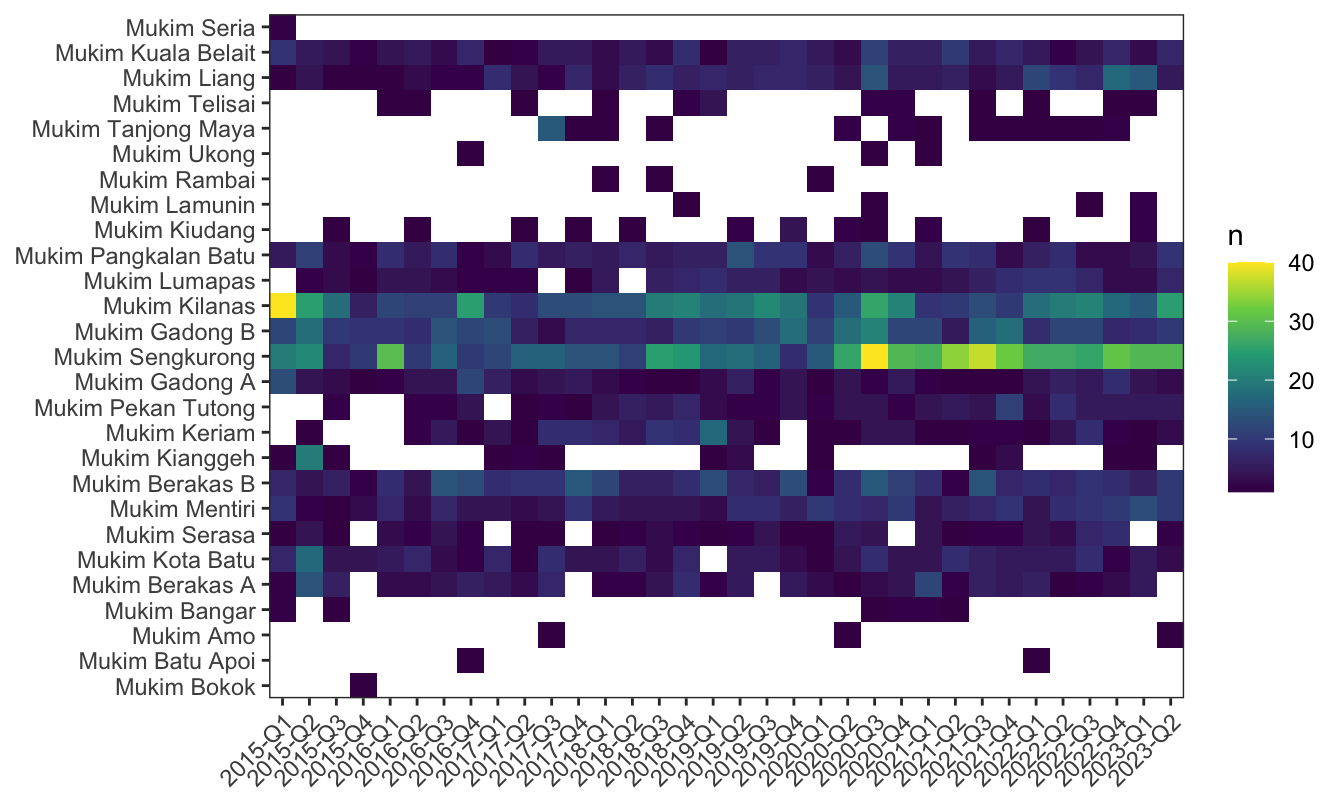
For analysis purposes, data aggregation at the desired spatial and temporal scales is essential, employing central tendency measures to typify the average property characteristics per mukim per time period. Continuous variables are summarized using either the median or mean, depending on the skewness of the data distribution, while the mode is applied for categorical variables. This aggregation process, however, highlights data sparsity across numerous mukims with absent transactions in specific periods (Figure 2). The need to impute the data set prior to modelling is therefore necessary, and is discussed in Section 4.3.

Figure 2: Sample size distribution among mukim and quarters. Empty cells indicate no recorded transactions.

3.3 Preliminary data analysis

Table 1 provides the summary statistics for the study variables. The main response variable that we are interested in is the sale price of the property, reported here in Brunei dollars. The mean sale price is BND 272,223 while the median is BND 255,000. The mean and median prices are quite different, suggesting that the distribution of sale prices is skewed, which is quite common for price data.

Table 1: Summary statistics for the property transaction data

Variable	N = 3,763	Missing (%)	Mean (SD)	Median (IQR)	Range
		0 (0%)	272 (123)	255 (200, 320)	24 - 2,006
		6 (0.2%)
	1,968 (52%)
	700 (19%)
	708 (19%)
	310 (8.3%)
	71 (1.9%)
		386 (10%)	2,400 (1,133)	2,284 (1,722, 2,798)	0 - 19,646
		447 (12%)	4 (1)	4 (3, 4)	0 - 12
		449 (12%)	4 (1)	3 (3, 4)	0 - 16
		370 (9.8%)	0.28 (0.60)	0.12 (0.07, 0.21)	0.01 - 5.19
		0 (0%)
	2,812 (75%)
	817 (22%)
	134 (3.6%)

The private residential property market in Brunei consists of a range of options such as apartments, townhouses, and detached houses (Hassan, 2023). The five categories considered in this data set are detached (52%), demi-detached (19%), terrace (19%), apartment (8%), and vacant land (2%). Evidently, the majority of transactions are landed property, with detached houses being the most commonly transacted property type. Besides the prevalence of multi-generational households, it could be argued that the demand for detached houses in Brunei is also fuelled by their contribution to socio-economic development, such as homestay initiatives (Janaji & Ibrahim, 2020).

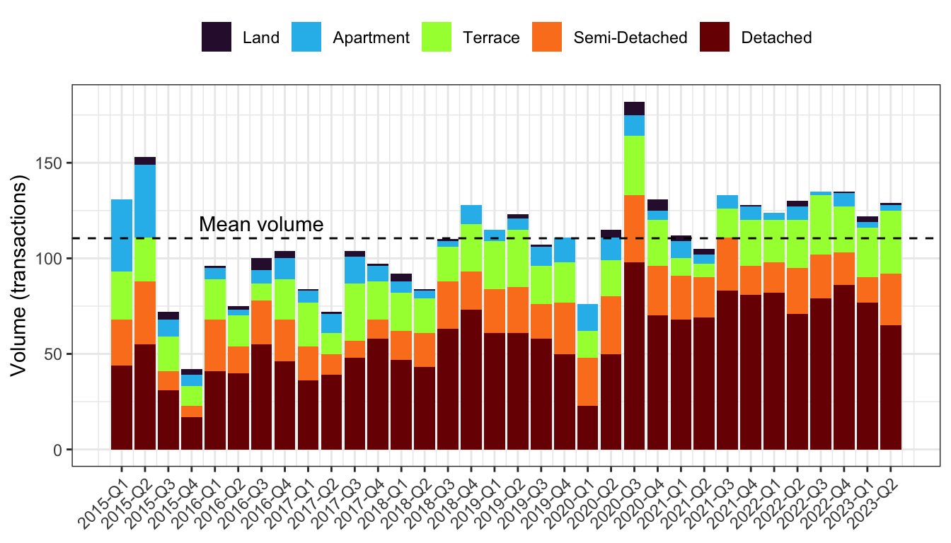
On the flip side, the demand for apartments is relatively low, and this is consistent with the findings of Hassan et al. (2011). The reluctance to embrace apartment living stems from unmet cultural and lifestyle needs within high-density complexes, despite government efforts to promote vertical living as a solution to land scarcity and urban sprawl. From Figure 3, we in fact see a declining pattern in the sales of apartments over time, and the dominant property type is detached houses.

Figure 3: Volume of property transactions by type over time.

In terms of specific property characteristics, averaging across mukims and time periods, we find that the median built-up area is 2,284 square feet (212 square metres), giving an indication of the size of the typical house in Brunei. Such a size is logically associated with a two-storey house, comprising of 3-4 bedrooms and a similar number of bathrooms, and this is indeed the case (Table 1).

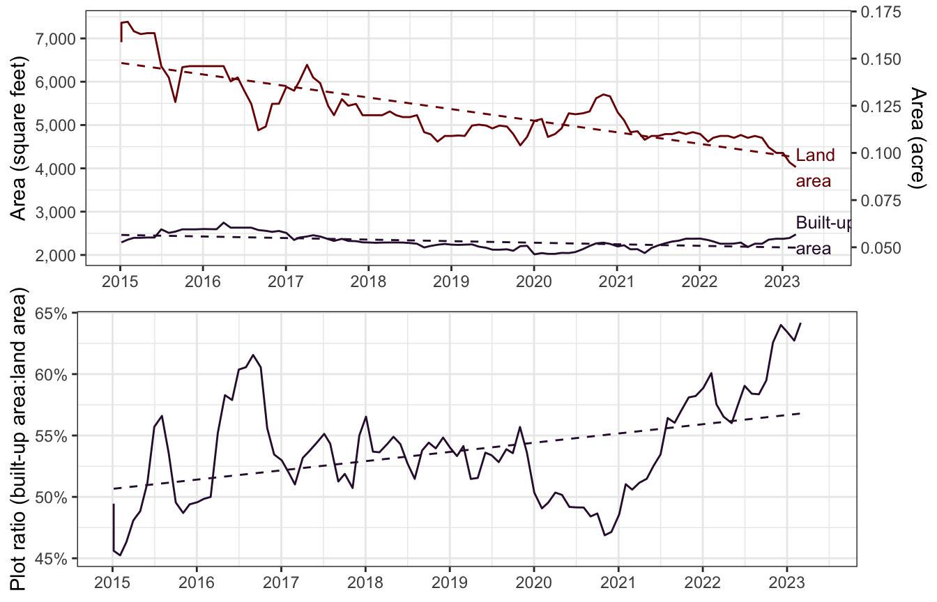
The median land area that was purchased is 0.121 acres (490 square metres). Land sizes bought seem to be decreasing over time, as seen in Figure 4. Combining this fact with the trend of built-up areas, it does seem that plot ratios² are increasing over time, from about 50% in 2015, to 63% in 2023. This is further corroborated by the 2021 census (DEPS, 2022), where a two-fold increase in semi-detached and terrace ownerships was reported.

Figure 4: Median land size and built-up area (top) and plot ratios (bottom) over time.

As noted by Hassan (2023), mukims do influence property prices as they denote distinct regions within the districts, with variations in prices across mukims attributed to differences in location, available amenities, and market demand. Table 2 tabulates, in decreasing order, the volume of transactions recorded during the data collection period across different mukims. Out of the total 39 unique mukims in Brunei, only \(M=27\) were recorded in the data set. This means the remaining 12 mukims, which comprise of areas in Kampong Ayer (water villages) and reserved forests, did not have any transactions during the data collection period, as is expected.

Table 2: Volume of transactions and the corresponding median price by mukim

	Mukim	District	Median Price (BND)	Sales Volume
1	Mukim Sengkurong	Brunei Muara	$268,000	726 (19.3%)
2	Mukim Kilanas	Brunei Muara	$250,000	568 (15.1%)
3	Mukim Gadong B	Brunei Muara	$290,000	373 ( 9.9%)
4	Mukim Berakas B	Brunei Muara	$298,000	285 ( 7.6%)
5	Mukim Pangkalan Batu	Brunei Muara	$209,000	215 ( 5.7%)
6	Mukim Mentiri	Brunei Muara	$244,614	213 ( 5.7%)
7	Mukim Liang	Belait	$270,000	199 ( 5.3%)
8	Mukim Kuala Belait	Belait	$320,000	172 ( 4.6%)
9	Mukim Kota Batu	Brunei Muara	$326,000	170 ( 4.5%)
10	Mukim Lumapas	Brunei Muara	$199,500	138 ( 3.7%)
11	Mukim Berakas A	Brunei Muara	$276,630	134 ( 3.6%)
12	Mukim Gadong A	Brunei Muara	$300,000	130 ( 3.5%)
13	Mukim Keriam	Tutong	$176,400	116 ( 3.1%)
14	Mukim Pekan Tutong	Tutong	$190,000	114 ( 3.0%)
15	Mukim Serasa	Brunei Muara	$225,500	78 ( 2.1%)
16	Mukim Kianggeh	Brunei Muara	$223,700	37 ( 1.0%)
17	Mukim Tanjong Maya	Tutong	$116,250	30 ( 0.8%)
18	Mukim Kiudang	Tutong	$137,000	19 ( 0.5%)
19	Mukim Telisai	Tutong	$252,000	18 ( 0.5%)
20	Mukim Bangar	Temburong	$145,000	9 ( 0.2%)
21	Mukim Lamunin	Tutong	$185,000	5 ( 0.1%)
22	Mukim Amo	Temburong	$85,000	3 ( 0.1%)
23	Mukim Rambai	Tutong	$50,500	3 ( 0.1%)
24	Mukim Ukong	Tutong	$180,000	3 ( 0.1%)
25	Mukim Batu Apoi	Temburong	$105,193	2 ( 0.1%)
26	Mukim Seria	Belait	$177,500	2 ( 0.1%)
27	Mukim Bokok	Temburong	$38,000	1 ( 0.0%)

The data reveals that the three highest-volume transaction mukims, accounting for 44% of all transactions, are all situated in the Brunei-Muara district and are adjacent to one another, indicating a clustering effect. Moreover, among the top ten mukims by transaction volume, eight are in the Brunei-Muara district, with the other two in the Belait district. An examination of median prices shows that properties in Brunei-Muara and Belait districts command higher prices, while those in Tutong and Temburong districts are generally more affordable. While these observations don’t control for the specific features of the properties, which will be analysed in the upcoming modelling phase, they offer an initial insight into the spatial patterns of property prices across Brunei.

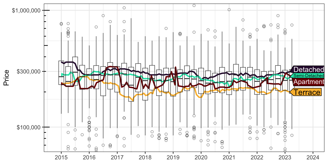
The data has also been organised into \(T=34\) quarterly time periods (2015 Q1 to 2023 Q2). The variability in property prices over time is illustrated in Figure 5, with boxplots revealing fluctuations in house prices across different periods. Median trend lines for detached, semi-detached, terraced houses, and apartments, smoothed using a 12-month rolling window, are also presented. Although it’s not immediately evident whether there’s a definitive trend in property prices over time from this preliminary analysis, further investigation will be undertaken during the modelling phase. Notably, apartment prices exhibit the most significant fluctuations, possibly reflecting the market’s reaction to shifts in the socio-demographic landscape, as previously discussed.

Figure 5: Property price trends over time. The boxplots show the distribution of prices for all property types. Individual trend lines (median smoothed using 12-month rolling window) are shown for detached, semi-detached, terraced houses, as well as apartments.

4 Methods

This section provides detailed descriptions of the methods used to analyse the data, including the statistical tests and models employed.

4.1 Statistical tests

An aim of bivariate analysis may be to determine whether a continuous or categorical study variable’s distribution varies across different categories. For continuous study variables, the Kruskal-Wallis test checks if the medians differ across three or more groups when data don’t meet normality, serving as a non-parametric counterpart to ANOVA. For categorical study variables, Fisher’s exact test evaluates the association in a contingency table, calculating the precise probability of the observed data under the null hypothesis of no association, with bootstrapping as a computational method for large tables. To assess the relationship between two continuous variables on the other hand, the Pearson test is often used to identify linear relationships. When the normality assumption is violated, the Spearman rank correlation test is employed instead. Finally, the Kolmogorov-Smirnov test compares two samples to see if they come from the same distribution, focusing on the maximum difference in their distribution functions, with large p-values indicating insufficient evidence to reject the hypothesis of a common distribution.

4.2 Global tests for spatial and temporal autocorrelation

For areal data indexed by \(i=1,\dots,M\), the Moran (1948)’s I test is used as a measure of global spatial heterogeneity and overall clustering of the spatial data. The Moran’s I test statistic is defined by \[ I = \frac{M}{\sum_{i=1}^M\sum_{j=1}^M w_{ij}}\frac{\sum_{i=1}^M\sum_{j=1}^M w_{ij}(x_i-\bar x)(x_j-\bar x)}{\sum_{i=1}^M(x_i-\bar x)^2} \in [-1,1], \tag{6}\] where \(x_i\) is the value of the study variable for area \(i\), \(\bar x\) is the mean of the study variable, and \(w_{ij}\) is the spatial weight between areas \(i\) and \(j\). Values of \(I\) close to 1 (c.f. -1) indicate positive (c.f. negative) spatial autocorrelation, whereas values close to 0 indicate no spatial autocorrelation. The null hypothesis of \(I=0\) is often compared against an alternative of \(I>0\). Under \(H_0\), the mean and variance of \(I\) have closed form expressions, and the Central Limit Theorem is invoked to calculate p-values based on a \(Z\) score.

In practice however, the normality assumption is not always met. In such cases, the permutation test is used to calculate p-values. This involves shuffling the values of the study variable across the spatial units, and recalculating the Moran’s I test statistic repeatedly (Cliff & Ord, 1981). The p-value is then calculated as the proportion of times the permuted test statistic exceeds the observed test statistic.

To test for temporal autocorrelations, the Ljung-Box test (Ljung & Box, 1978) can be used. This primarily checks the absence of serial correlation in the residuals of a time series. The null hypothesis is stated as “the data are independently distributed”, which is then tested against an alternative of “the data exhibit autocorrelation”. The test statistic is calculated using the formula \[ Q = n(n+2) \sum_{k=1}^h \frac{\hat\rho_k^2}{n-k}, \] where \(n\) is the sample size, \(h\) is the number of lags being tested, and \[ \hat\rho_k = \frac{\sum_{t=k+1}^n (x_t-\bar y)(x_{t-k}-\bar x)}{\sum_{t=1}^n (x_t-\bar x)^2} \in[-1,1] \] is the sample (auto)correlation between a series and its lagged values. The \(Q\) test statistic is then referred to the chi-square distribution.

To apply either the Moran’s test or the Ljung-Box test, the rectangular \(M\times T\) data set (depicted in Figure 2) must be flattened vertically or horizontally into a single vector that varies either across space or time respectively. Thus, when testing for spatial autocorrelation the temporal dimension is ignored, and vice versa. To account for both dimensions at the same time, a variation of the Moran’s I test found in Bian-Ling (2014) is proposed, one that incorporates the temporal dimension simultaneously with the spatial dimension.

Let \(\mathbf x=(x_{mt}) \in \mathbb R^{MT}\) be the vectorised data set, with indices for space (\(m=1,\dots,M\)) running faster than those for time (\(t=1,\dots,T\)). Notice that the Moran’s test (Equation 6) can be written in Matrix form: \[ I = \frac{\dim(\mathbf x)}{\mathbf 1^\top \tilde{\mathbf W} \mathbf 1} \frac{(\mathbf x - \bar {\mathbf x})^\top \tilde{\mathbf W} (\mathbf x-\bar {\mathbf x})}{(\mathbf x-\bar {\mathbf x})^\top (\mathbf x-\bar {\mathbf x})}, \tag{7}\] where \(\tilde{\mathbf W}\) is a weight matrix of appropriate size. The following weight matrix is proposed: \[ \tilde{\mathbf W} = (\mathbf I + \mathbf D) \otimes \mathbf W, \tag{8}\] where the ‘\(\otimes\)’ operator is the Kronecker product of two matrices, \(\mathbf I\) the identity matrix, and \(\mathbf D=(d_{tt'})_{t,t'=1}^T\) is the temporal weight matrix defined by: \[ d_{tt'} = \begin{cases} 1 & \text{if } |t-t'| = 1,\\ 0 & \text{otherwise.} \end{cases} \tag{9}\] This is a simple design matrix that structures the temporal dependencies in the data by linking each adjacent time points (time lag of 1). Typically (spatial) weight matrices dictate that the diagonal entries be zero, since by definition a spatial unit cannot be its own neighbour. In this case, the diagonal elements are set to 1 (by adding the identity matrix to \(\mathbf D\)) to account for the spatial dependencies in the same time point. More complex time dependencies are able to be modelled (e.g. increased time lags or kernel-based weights) by altering the structure of \(\mathbf D\).

4.3 Spatio-temporal models

Let \(Y_{mt}\) denote the observed property price for area \(m\in\{1,\dots,M\}\) at time period \(t=1,\dots,T\). In addition to the property prices, we also have area-level covariates which are temporally distributed as per those listed in Table 1. Collectively denote the covariates relating to area \(m\) at time period \(t\) as \(\mathbf X_{mt}^\top = (X_{1,mt}, \dots, X_{p,mt})\).

The main idea of spatio-temporal models is to be able to encode the spatial and temporal effects into the modelling process. As a spin-off to the CAR class of models, the linear regression model (Equation 1) is modified to include a latent spatio-temporal random effect \(\psi_{mt}\) as a linear predictor. Specifically, the linear model becomes \[ \begin{gathered} Y_{mt} = \beta_0 + \beta_1X_{1,mt} + \cdots + \beta_pX_{p,mt} + \psi_{mt} + \epsilon_{mt} \\ \epsilon_{mt} \sim \operatorname{N}(0,\sigma^2). \end{gathered} \tag{10}\] The errors are independently and identically normal conditional on observing the value of \(\psi_{mt}\). These latent effects \(\psi_{mt}\) are further decomposed into spatial and temporal components, so that the each can be quantified separately. The spatial component can be modelled using the CAR prior (Equation 5), while the temporal component can be handled in several ways. Three are described in this article: 1) The linear effect of time, 2) the ANOVA decomposition, and 3) the time autoregressive process.

4.3.1 Linear time model

Modelling a linear effect of time allows us to estimate the autocorrelated time trends for each areal unit, thereby estimating areas exhibiting changing linear trends in response over time (Bernardinelli et al., 1995). The linear time model is \[ \begin{gathered} \psi_{mt} = \phi_m + (\alpha + \delta_m)t \\ \phi_m \mid \boldsymbol \phi_{-m} \sim \operatorname{CAR}(\mathbf W,\rho_1, \tau^2_1) \\ \delta_m \mid \boldsymbol \delta_{-m} \sim \operatorname{CAR}(\mathbf W,\rho_2, \tau^2_2) \end{gathered} \tag{11}\]

There are two main features of this linear time model. Firstly, this model facilitates the estimation of a spatially varying intercept \(\beta_0 + \phi_k\), where the \(\beta_0\) is the grand intercept coming from the coefficients in the linear predictor \(\boldsymbol\beta\). This allows average response variables to vary across space, while accounting for spatial dependencies. Secondly, the model also estimates spatially varying time slopes. Reminiscent of growth models, this allows for the study a linear temporal trend in the response variables, both globally (\(\alpha\) parameter) and locally within each spatial area (\(\delta_m\) parameter).

4.3.2 ANOVA decomposition

This model decomposes the spatio-temporal variation into its constituent parts of space (\(\phi_m\)) and time (\(\delta_t\)), with the goal being to estimate the overall time trends and spatial patterns exhibited by the data (Knorr-Held, 2000). No assumption is made regarding the functional form of time (linear or otherwise). The model is \[ \begin{gathered} \psi_{mt} = \phi_m + \delta_t \\ \phi_m \mid \boldsymbol \phi_{-m} \sim \operatorname{CAR}(\mathbf W, \rho_S, \tau^2_S) \\ \delta_t \mid \boldsymbol \delta_{-t} \sim \operatorname{CAR}(\mathbf D, \rho_T, \tau^2_T) \end{gathered} \tag{12}\]

In this ANOVA model, both the autocorrelation of the spatial and temporal effects are governed by the CAR prior with their own set of \((\rho,\tau)\) parameters. Here, the temporal adjacency matrix \(\mathbf D\), defined as in (Equation 9), is used in the CAR prior for \(\delta_t\). The addition of a time-space interaction effect, \(\gamma_{mt}\sim\operatorname{N}(0,\tau_I^2)\) say, is possible for non-Gaussian likelihoods. However, for the Gaussian model, this parameter is not identifiable with the model errors \(\epsilon_{mt}\).

4.3.3 Time autoregressive models

It is possible to estimate evolution of spatial random effects over time by considering autoregressive (AR) structure of time of order up to 2 (Rushworth et al., 2014). As is common with AR models, the dependence of time is built into the model in such a way that the observation at any time point \(t\) is dependent also on previous observations. Let us say \(\psi_{mt} = \phi_{mt}\), and define the spatial effects vector to be \(\boldsymbol\phi_t=(\phi_{1t},\dots,\phi_{Mt})^\top\) for each time point. Then a vector autoregressive model is \[ \begin{gathered} \boldsymbol\phi_{t} \mid \boldsymbol\phi_{t-1}, \boldsymbol\phi_{t-2} \sim \operatorname{N}_M\left( \rho_1 \boldsymbol\phi_{t-1} + \rho_2 \boldsymbol\phi_{t-2}, \tau^2 \mathbf Q(\mathbf W, \rho_S)^{-1} \right) \\ \boldsymbol\phi_{1} \sim \operatorname{N}_M\left( \mathbf 0, \tau^2 \mathbf Q(\mathbf W, \rho_S)^{-1} \right), \end{gathered} \tag{13}\] where the precision matrix \(\mathbf Q\), as a function of the spatial weights \(\mathbf W\) and a spatial dependence parameter \(\rho_S\), is given as per Leroux et al. (2000): \[ \mathbf Q(\mathbf W, \rho_S) = \rho_S\left( \operatorname{diag}\big(\textstyle\sum_k w_{kj}\big)_{j=1}^M - \mathbf W \right) + (1-\rho_S) \mathbf I_M. \] It can be shown, using Brook’s lemma, that this corresponds to the precision matrix of the joint distribution of the conditional spatial effects discussed earlier in (Equation 5) For this model, temporal autocorrelation is induced by the mean, while the spatial autocorrelation is induced by the variance (Lee et al., 2018). The temporal autocorrelation is controlled by the \(\rho_1\) and \(\rho_2\) parameters, which are each constrained between 0 and 1 to ensure stability and stationarity.

4.3.4 Model estimation

Model estimation is done using Bayesian methods, where additional priors need to be chosen on the parameters to be estimated. For the present study, I default to the uninformative priors, i.e. uniform priors for \(\rho\), \(\Gamma^{-1}(1, 0.01)\) priors for variance/scale parameters, and independent flat normal priors for the coefficients. This happens to be the default choices in the {CARBayesST} R package (Lee et al., 2018) that is used to fit the models.

Inference is conducted on the posterior distribution of the parameters (e.g. posterior mean and 95% credible intervals). Posterior sampling is done by way of Markov chain Monte Carlo (MCMC) methods. All parameters whose full conditional distributions have a closed form distribution are Gibbs sampled (e.g. the regression coefficients \(\boldsymbol\beta\), the random effects \(\boldsymbol\phi\), and variance parameters). Remaining parameters are updated using Metropolis or Metropolis-Hastings steps. Convergence is assessed by visual checks and using the convergence diagnostic proposed by Geweke (1992).

For model comparison purposes, the marginal log-likelihood value can be a useful metric, but they are not able to capture model complexities. Information criteria that penalises log-likelihood values based on the number of effective parameters, thereby giving preference to more parsimonious models. Examples include the Deviance Information Criterion (DIC) (Spiegelhalter et al., 2002) the Watanabe-Akaike Information Criterion (WIC) (Watanabe & Opper, 2010) (small values indicate better fit). Lastly, the log marginal predictive likelihood (LPML, Congdon, 2005) measures the ability of the model to predict new data using cross-validation techniques (higher values indicate better fit).

4.4 Spatio-temporal imputation

For the spatio-temporal models described above, the presence of missing data can be problematic if not treated properly. A complete case analysis will exclude spatial areas with missing covariates, potentially losing valuable information. If it can be shown that On the other hand, a naïve imputation method that does not respect the spatio-temporal structure of the data can introduce bias and reduce the precision of the estimates.

Missingness in the data is likely to be missing at random (MAR) – as the probability of missingness is directly related to its spatial location (Rubin, 1976). This is true when considering certain areas are much less likely to be purchased, and thus less likely to be have full information regarding it. The method that is proposed here is a simple mean imputation that respects the spatio-temporal structure of the data, extending the interpretation of Tobler’s first law of geography³ to time as well as space. The imputation strategy is laid out in Algorithm 1.

\begin{algorithm} \caption{Spatio-temporal mean imputation} \begin{algorithmic} \State \textbf{input:} Raw data $\mathbf X$, Neighbourhood structure $\mathcal N$ \State \textbf{output:} Imputed $\tilde{\mathbf X}$ \Procedure{STMeanImputation}{$\mathbf X$, $\mathcal N$} \For{$m=1,\dots,M$} \State $\mathcal N(m) \leftarrow$ Spatial neighbours of $m$ \State $\mathbf X_m\leftarrow \{\mathbf X \text{ at location } k \mid k \in \mathcal N(m)$\} \If{$\mathbf X$ continuous} \State $\tilde{\mathbf X}_m\leftarrow$ 3-quarter rolling window \Call{Mean}{} or \Call{Median}{} \EndIf \If{$\mathbf X$ discrete} \State $\tilde{\mathbf X}_m\leftarrow$ 3-quarter rolling window \Call{Mode}{} \EndIf \EndFor \State $\tilde{\mathbf X}\leftarrow (\tilde{\mathbf X}_1,\dots,\tilde{\mathbf X}_M)$ \Return $\tilde{\mathbf X}$ \EndProcedure \State \State $\tilde{\mathbf X}\gets$ \Call{STMeanImputation}{$\mathbf X$, $\mathcal N$} \While{$\tilde{\mathbf X}$ is not complete} \State $\tilde{\mathbf X}\leftarrow$ \Call{STMeanImputation}{$\tilde{\mathbf X}$, $\mathcal N$} \EndWhile \end{algorithmic} \end{algorithm}

In essence, the algorithm iteratively imputes missing values by taking the mean, median, or mode of the values of the spatial neighbours. A 3-quarter rolling window is used to smooth the imputed values and borrow strength from the adjacent time points. The process is repeated until there are no missing values in the data set. The imputation may be validated by visually and statistically testing the distribution of the original data set with the imputed data set to ensure that the imputation process has not introduced any significant bias.

Finally, it is noted that the response variable (property price) need not undergo this spatio-temporal imputation process, as this will be handled directly by the Bayesian models described above. Missing response variables will be imputed automatically using the posterior distribution of the response variable given the observed covariates and the spatial and temporal structure of the data during the model fitting phase.

5 Results

The results section is split into three parts: bivariate analysis, imputation, and model fit.

5.1 Bivariate analysis

At the outset, examining how the main response variable vary with other study variables can guide the selection of covariates for our model. Summary statistics in Table 3 highlight the variation in property prices and other variables by property type. All differences found in the table are statistically significant (p<0.001), and the analysis remains valid even when the data set is filtered to remove the “Land” type data points (of which there are only N=71).

There is indeed a marked difference in prices among property types (p<0.001). Detached houses emerge as the most expensive, with a median price of BND 288,000, followed by semi-detached houses, apartments, and terraced houses. Notably, detached, semi-detached, and apartments show prices in the upper quartile exceeding BND 300,000, while terraced houses have an upper quartile price of BND 250,000.

The interaction between property type and other variables presents intriguing insights. For instance, landed properties average a built-up area of 2,100–2,500 square feet, while apartments average only 1,700 square feet. This fact, combined with the relatively expensive prices for apartments, makes apartments less appealing in terms of price per square foot.

Additionally, Table 3 details the average land size for each property type. Detached houses average 0.15 acres, significantly larger than the land for semi-detached (0.08 acres) and terraced houses (0.05 acres). Despite the similar built-up area across these landed properties, semi-detached and especially terraces offer less outdoor space, a compromise for home owners. Yet, the prevalence of these more compact houses is growing, likely due to their lower cost per square foot.

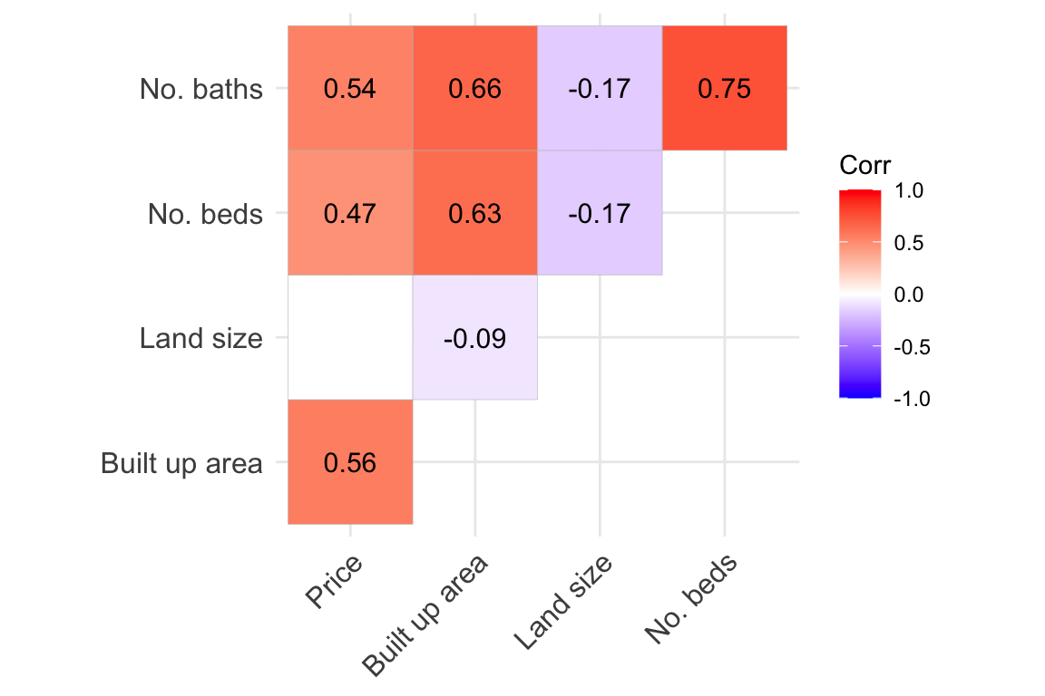
Shifting our attention to the correlations among continuous variables, the correlation plot (Figure 6) reveals that property prices positively correlate with all other continuous variables, except for land size. This pattern suggests that the physical size of the property is a critical factor in determining its price, rather than the size of the land it occupies. The strong correlation between the number of bedrooms and bathrooms is expected, as both are positively related to the built-up area. Interestingly, a negative correlation is observed between land size and built-up area. This seems to tie in with the earlier observation of increasing plot sizes. On the other hand, apartments typically report larger land sizes due to communal areas, potentially skewing this relationship. In any case, this negative correlation is quite small.

Table 3: Summary statistics for the property transaction data by property type

Characteristic	Detached, N = 1,9681	Semi-Detached, N = 7001	Terrace, N = 7081	Apartment, N = 3101	Land, N = 711	p-value2
Price (BND 1,000)	288 (220, 360)	267 (217, 301)	210 (171, 250)	233 (210, 300)	96 (68, 168)	<0.001
Built up area (sqft)	2,550 (2,025, 3,142)	2,264 (1,711, 2,744)	2,142 (1,785, 2,400)	1,672 (1,316, 1,709)	0 (0, 0)	<0.001
Price per sqft (BND)	113 (89, 136)	114 (98, 134)	100 (84, 118)	152 (136, 186)		<0.001
Land size (acre)	0.15 (0.11, 0.22)	0.08 (0.06, 0.10)	0.05 (0.04, 0.07)	1.02 (0.45, 2.91)	0.33 (0.21, 0.39)	<0.001
Price per 0.1 acre (BND 1,000)	199 (130, 270)	313 (221, 390)	384 (268, 475)	26 (10, 56)	38 (21, 54)	<0.001
Land type						<0.001
Freehold	1,689 (86%)	501 (72%)	534 (75%)	23 (7.4%)	59 (83%)
Leasehold	276 (14%)	187 (27%)	171 (24%)	171 (55%)	12 (17%)
Strata	3 (0.2%)	12 (1.7%)	3 (0.4%)	116 (37%)	0 (0%)
1 Median (IQR); n (%)
2 Kruskal-Wallis rank sum test; Fisher’s Exact Test for Count Data with simulated p-value (based on 2000 replicates)

Figure 6: Correlation plot of the study variables. Correlations which were not found to be significant using the Spearman correlation test are left blank.

5.2 Imputation

As a preliminary step to the imputation process, the data set is checked for spatial and temporal autocorrelation. The purpose is to establish the need for spatial imputation and that the subsequent spatio-temporal imputation process is justified.

Spatial autocorrelation is assessed using Moran’s I test across all study variables, with categorical variables such as property type and land type numerically coded for this purpose. The results show significant p-values for all variables, suggesting positive spatial autocorrelation, except for the property type variable, which shows a non-significant p-value (p=0.8). This might be attributed to the categorical nature of the property type variable, hinting that Moran’s I test might not be the most suitable for this variable.

For temporal autocorrelation, the Ljung-Box test is applied, with type and land type variables again numerically coded. The test was unable to return valid results for the beds and land type variables because there was virtually zero temporal variation in the data set. However, significant results for built up area and land size, which provide further evidence of the trend of increasing plot ratios over time (Figure 4). Despite the baths variable not showing significance, it is still included in the imputation due to its positive correlation with built-up area. Although the price variable is not significant–a point warranting further analysis in the modelling phase–it is not included in the imputation as the response variable is not part of the imputation process.

Table 4: Results for the Moran’s I test and Ljung-Box test for spatial and temporal autocorrelations.

Variable	Moran's I		Ljung-Box
	Statistic	p-value	Statistic	p-value
Price	0.431	0.001**	11.517	0.2
Type	−0.139	0.8	0.398	>0.9
Built up	0.214	0.032*	31.794	<0.001***
Beds	0.238	0.022*
Baths	0.183	0.053.	5.486	0.7
Land size	0.198	0.030*	41.502	<0.001***
Land type	0.147	0.085.

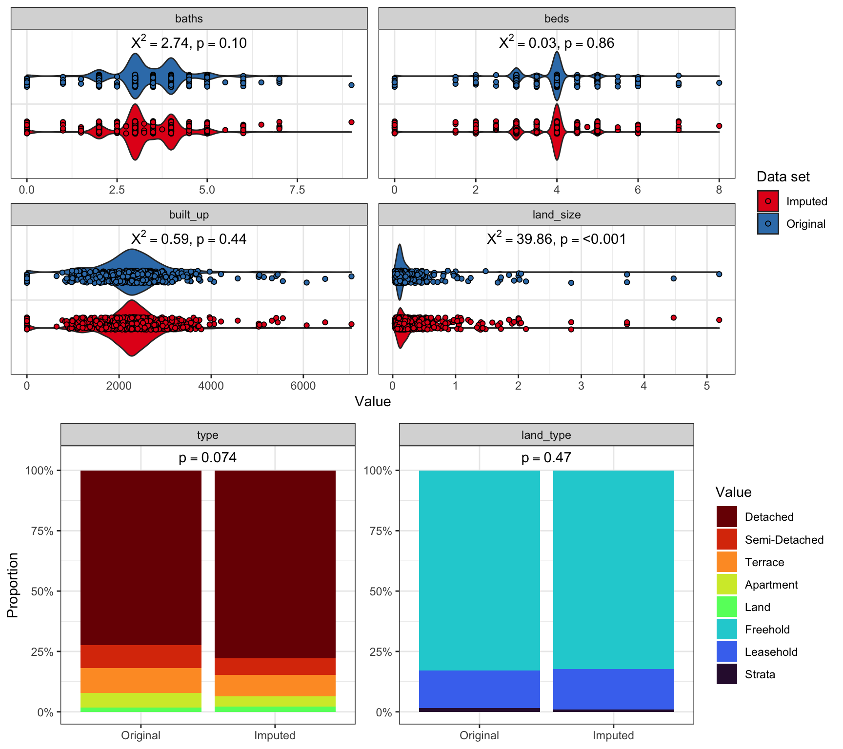
The spatio-temporal imputation process was carried out successfully, and a complete non-empty data set was obtained after two imputation cycles. To evaluate the imputation’s effectiveness, Figure 7 displays the distribution between the original and imputed datasets for comparison, and reports the Kolmogorov-Smirnov test of the difference. The inability to reject the null hypothesis suggests no significant differences between the two datasets for most variables. Specifically for the continuous variables, baths, beds, and built-up area align closely with their original values, whereas land size shows some notable differences. This discrepancy likely stems from the high variability in land size not adequately accounted for by property type during imputation, as evidenced by an increase in 1-2 acre properties in the imputed data.

For the categorical variables (type and land type), there’s no significant deviation from the original dataset at a 5% significance level. However, the type variable’s Kolmogorov-Smirnov p-value of 0.074 approaches significance, hinting at a slightly higher proportion of detached houses and vacant lands in the imputed data, which can be seen visually in the plot.

While the imputation process generally reflects the original dataset accurately, areas requiring refinement have been identified, particularly with land size variability and categorical variable proportions. These points will be further explored in the conclusion section.

Figure 7: Comparison of the imputed data set with the original data set. The p-values are from the Kolmogorov-Smirnov test.

5.3 Model fit

Seeing that land type properties are markedly dissimilar from the other property types, it would be wise to account for this explicitly in the model. The spatio-temporal model that will be fit is the following: \[ Y_{mt} = \begin{cases} \\ \beta_0 + \beta_1 \texttt{type} + \beta_2\texttt{built\_up} + \beta_3\texttt{beds} \\ + \beta_4\texttt{baths} + \beta_5\texttt{land\_size} + \beta_6\texttt{land\_type} \hspace{1em} &\texttt{type}\neq\texttt{"Land"} \\ + \psi_{mt} + \epsilon_{mt} \\ \\ \beta_0 + \beta_5\texttt{land\_size} + \beta_6\texttt{land\_type} &\texttt{type}=\texttt{"Land"} \\ + \psi_{mt} + \epsilon_{mt} \\ \\ \end{cases} \] This can be achieved by having an interaction between a dummy variable for land type, and the built up area, beds, and baths variables. Zeroing out these values in the rows of the data where the property type is land will also have the same effect.

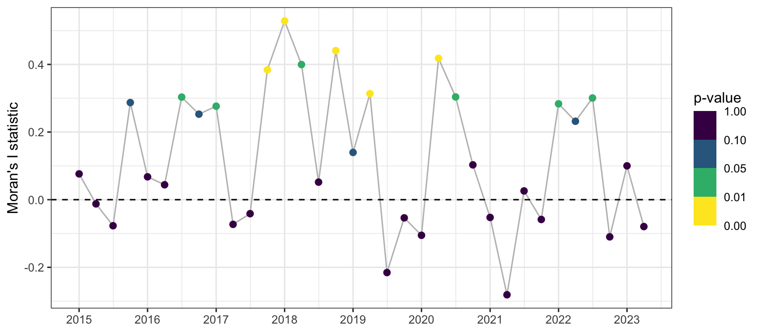
After initially fitting an ordinary linear regression model (referred to as M0), its residuals are examined for spatial and temporal autocorrelation. Following Lee et al. (2018), the data set is treated as spatial panel data, with Moran’s test applied to each time period to assess autocorrelation. The Moran’s I statistics, as shown in Figure 8, predominantly exceed zero, indicating positive spatial autocorrelation. However, less than half of these results are statistically significant, complicating the interpretation of these findings. Additionally, this method requires reducing the panel data to only \(M=27\) data points for each time period.

Figure 8: Spatio-temporal Moran tests

Using the proposed global spatio-temporal Moran’s test described in Section 4.2, a significantly positive value for the test statistic is observed (I = 0.142, p = <0.001). This gives an indication that the ordinary linear regression model is not able to sufficiently capture the spatio-temporal heterogeneity in the price variable even when controlled by covariates.

Based on the above information, four CAR-based spatio-temporal models are fitted: the linear time model (M1), the ANOVA model (M2), and the time AR(1) and AR(2) models (M3 and M4, respectively). The results of the model fit are shown in Table 5. For each model, 1,500,000 MCMC samples were obtained, and the first 500,000 samples discarded as burn-in. The remaining samples were thinned by a factor of 100, yielding a total of 10,000 samples used for inference. All diagnostics for the MCMC chains were satisfactory, and the Gelman-Rubin statistic was close to 1.0 for all parameters.

Not surprisingly, Model M0 demonstrates the poorest fit among the models tested. The inclusion of spatial effects leads to a notable decrease in error variance, underscoring the linear model’s failure to encompass the spatio-temporal heterogeneity of the price variable, instead attributing all discrepancies to the error term. The linear time model M1 and the ANOVA model M2 show a marked improvement in fit, as evidenced by reduced DIC and WAIC values. The AR(2) spatio-temporal model M4 appears to provide the best fit, though its DIC and WAIC values are not too different from those of the AR(1) model M3, particularly when considering the LPML statistic. The estimation of the temporal autoregressive parameter \(\rho_{1,T}\) approaching the upper limit of 1.0 in the AR(1) model suggests an attempt to capture a level of persistence in the time series that exceeds the model’s constraint. A boundary estimate implies a strong temporal dependency, potentially hinting at the model’s inclination to express an even stronger relationship. Consequently, the AR(2) model is identified as the most appropriate choice to provide a better fit by accommodating greater persistence within the data’s temporal structure.

This suggests that the housing market in Brunei exhibits both spatial and temporal dependencies, necessitating an autoregressive model of order 2 to adequately represent the market’s temporal dynamics. Economically, this implies that the housing market potentially takes up to a period of two quarters (six months) to fully incorporate the effects of any changes or shocks. This stresses the importance of considering both recent and slightly older market conditions and regulatory adjustments when predicting property prices.

Interpreting model M4, we observe that all coefficients in the linear predictor are significant, with two exceptions. The first is the land type variable (and its associated dummy variables), where no significant difference in average price, holding other factors constant, is observed among different land types (freehold, leasehold, and strata titles). This could be attributed to a potential collinearity effect, as land types and property types are closely related; for instance, most apartments are strata titled, whereas detached houses are likely to be freehold. The second is the dummy variable for apartments, which indicates no significant difference in average price between apartments and the base category (vacant lands). However, the upper 95% confidence interval (CI) actually approaches 0, suggesting a possible rationale for retaining this variable in the model.

Table 5: Comparison of model fits.

	M0		M1		M2		M3		M4
	Coef.	95% CI	Coef.	95% CI	Coef.	95% CI	Coef.	95% CI	Coef.	95% CI
Coefficients
Intercept	231	[174, 288]*	191	[142, 240]*	190	[141, 239]*	180	[133, 227]*	176	[130, 222]*
Type (ref: Land)
Detached	−150	[-215, -83.4]*	−104	[-163, -49.6]*	−103	[-160, -46.6]*	−75.4	[-129, -21.9]*	−78.9	[-134, -25.2]*
Semi-Detached	−152	[-220, -82.7]*	−119	[-178, -62.0]*	−120	[-178, -61.8]*	−89.4	[-145, -33.6]*	−92.9	[-149, -37.3]*
Terrace	−177	[-246, -109]*	−152	[-211, -95.4]*	−153	[-211, -95.0]*	−111	[-167, -54.8]*	−114	[-170, -57.4]*
Apartment	−51.2	[-118, 15.8]	−83.1	[-141, -26.8]*	−84.7	[-141, -28.4]*	−51.7	[-105, 2.75]	−49.7	[-104, 3.40]
Built up area (1000 sqft)	22.7	[10.3, 35.0]*	18.2	[8.48, 28.1]*	16.6	[6.95, 26.4]*	19.3	[9.99, 28.6]*	20.0	[10.7, 29.2]*
No. of beds	5.66	[-7.53, 19.1]	12.7	[2.50, 22.9]*	13.0	[2.63, 23.3]*	10.3	[0.64, 20.1]*	11.0	[0.76, 21.0]*
No. of baths	27.6	[16.6, 38.4]*	14.9	[6.38, 23.6]*	15.5	[6.77, 24.0]*	14.6	[6.31, 23.1]*	14.6	[6.14, 23.0]*
Land area (0.1 acre)	−8.13	[-26.5, 9.78]	14.6	[0.32, 28.9]*	13.3	[-1.03, 27.6]	14.2	[0.15, 28.1]*	13.7	[0.15, 27.0]*
Land type (ref: Freehold)
Leasehold	18.6	[-1.22, 38.2]	1.46	[-18.7, 21.6]	2.04	[-17.4, 22.0]	0.427	[-19.0, 20.1]	1.19	[-18.0, 21.1]
Strata	92.9	[33.1, 153]*	37.1	[-10.3, 86.0]	38.6	[-8.89, 86.4]	7.85	[-38.0, 54.1]	3.51	[-42.8, 49.9]
Spatio-temporal parameters
\(\rho_S\)			0.501	[0.10, 0.91]*	0.486	[0.08, 0.91]*	0.398	[0.13, 0.75]*	0.430	[0.15, 0.69]*
\(\alpha\)			14.8	[-3.45, 33.2]
\(\rho_{1,T}\)			0.406	[0.02, 0.91]*	0.394	[0.02, 0.91]*	0.989	[0.97, 1.00]*	0.484	[0.27, 0.84]*
\(\rho_{2,T}\)									0.508	[0.15, 0.73]*
Variance parameters
\(\sigma^2\)	6,380	[5681, 7155]*	3,570	[3162, 4039]*	3,580	[3170, 4040]*	2,710	[2324, 3160]*	2,390	[1892, 2913]*
\(\tau^2_S\)			9,400	[4594, 17510]*	9,360	[4596, 17436]*
\(\tau^2_T\)			0.0161	[0.00, 0.09]*	0.0138	[0.00, 0.06]*
\(\tau^2\)							656	[390, 1040]*	1,480	[820, 2318]*
Model fit criteria
DIC \((p_d)\) 1	6,509	(11.9)	6,208	(36.6)	6,208	(35.5)	6,143	(126.3)	6,120	(175.5)
WAIC \((p_w)\) 1	6,524	(25.2)	6,224	(47.3)	6,224	(46.3)	6,160	(119.9)	6,140	(159.1)
LMPL	−3,262		−3,113		−3,113		−3,089		−3,090
Loglik.	−3,242		−3,067		−3,068		−2,945		−2,884
Asterisks (*) indicate that 0 is not within the 95% credible interval.
1 \(p_d\) and \(p_w\) are the estimated number of effective parameters.

The intercept in this model represents the estimated average price when all continuous variables are set to zero and categorical variables are at their reference levels. For our analysis, the intercept, valued at approximately BND 176,000, represents the “baseline value associated with owning freehold land”. The intercept could be fixed at zero when all attributes of a property is absent, but arguably this is too strong an assumption to make. This baseline value could encompass various minimum costs associated with constructing a liveable property, including planning permission, legal fees, and infrastructure expenses such as access roads, water, electricity, and high-speed broadband.

Accordingly, the property-specific average price ranking, in ascending order, is: terrace (BND 62,000), semi-detached (BND 83,000), detached (BND 97,000), apartment (BND 126,000). This ranking highlights the relatively poor value proposition of apartments. Another point to make is that the model makes a significant price differential between buying land and purchasing a ready-made property. The scarcity of land transactions supports this observation, possibly due to the challenges in securing financial loans for land purchases, which banks may view as riskier compared to ready-built properties.

Coefficients for built up area, number of beds and baths are all positive. This is expected, clearly, as larger properties logically command a higher price. This relationship is quantified as follows: For every 1000 square feet increase in built up area accompanied by the addition of an en suite bedroom, the price increases by approximately BND 46,000.

The spatial effect, with an estimated value of \(\rho=0.43\), highlights the degree of price dependency on neighbouring properties. A positive \(\rho\) indicates evidence of a clustering effect, which is seen here. Being significant at the 5% level, this observation reinforces the concept of geographical influence on property prices, even after controlling for other factors. In the time autoregressive models such as M3 and M4, the spatial effects are manifested through the estimation of the spatial random effect vector \(\boldsymbol\phi_t = (\phi_{1t},\dots,\phi_{Mt})^\top\), which are even separated temporally. Under a Bayesian paradigm, posterior estimates of \(\boldsymbol\phi_t\) may be obtained and examined if so desired.

The temporal autoregressive parameters for lag 1 and 2 are 0.48 and 0.51 respectively. Both of these effects are positive, which means that any current price point is expected to increase if past values increase as well, with effects from two prior time points affecting the current value almost equally. As the sum of these coefficients is less than 1, the impacts of any past shocks will gradually diminish over time rather than persist indefinitely or amplify.

5.4 Prediction of property prices

Table 6: The typical property characteristics in Brunei (for prediction purposes).

Characteristic	Value
Property type	Detached
Built up area (sqft)	2284.2
No. of beds	4
No. of baths	3
Land size (acre)	0.121
Land type	Freehold

In this section, the AR(2) model M4 will be used to predict property prices in Brunei to get a sense of the spatial and temporal dynamics of the housing market. The model will be used to predict the typical house price in Brunei, which, based on the previous preliminary data analysis in Section 3.3, is found to have the characteristics described in Table 6. These will be the (time-invariant) \(\mathbf X\) values and plugged into the Equation 13. Parameter values for the model are obtained from the posterior sample, thus allowing us to generate the posterior predictive distribution (Gelman, 2014) of the typical house in Brunei.

Figure 9: Predicted property prices in Brunei segregated by mukim and average across all time periods.

The map in Figure 9 overlays the predicted property prices for each mukim in Brunei, averaged across all time periods. According to the fitted model M4, the top three most expensive properties are located in Mukim Kianggeh (BND 486,000), Mukim Gadong A (BND 331,000), and Mukim Kuala Belait (BND 314,000). The cheapest properties are found in Mukim Rambai (BND 130,000), Mukim Amo (BND 140,000), and Mukim Kiudang (BND 162,000). Evidently, the spatial effect is quite pronounced, with the most expensive properties being clustered in the urban areas of Brunei-Muara and Kuala Belait districts, while the cheapest properties are located in the rural areas of Tutong and Temburong districts.

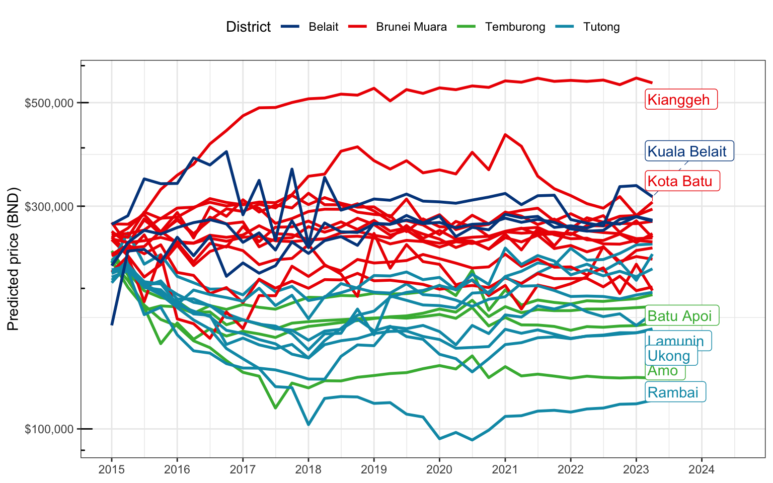
It is also possible to visualize the evolution of predicted property prices over time for each mukim (Figure 10). The period of 2015 to 2018 saw a diverging variability in property prices across mukims, with some mukims (Kianggeh, Kuala Belait, and Kota Batu) experiencing a sharp increase in prices while others experienced a sharp decrease (most mukims in Tutong and Temburong). From then onwards, the prices were relatively steady throughout. Perhaps most interesting is the sharp increase in the price for Mukim Kota Batu in 2018, coinciding with advanced stages of the construction of the Temburong Bridge in the vicinity.

Figure 10: Evolution of predicted property prices over time for each mukim.

6 Conclusions

This study has meticulously explored the spatial and temporal dynamics of property prices in Brunei, revealing pronounced spatio-temporal effects. The analysis underscores the necessity of robust modelling to draw valid inferences about the real estate market. Through the use of spatio-temporal Conditional Autoregressive (CAR) models, spatial effect present in the data have been quantified, enabling the prediction of area-specific property prices across Brunei. Furthermore, the investigation into the temporal aspect of property prices suggests an autoregressive nature with a lag of two quarters. This finding is pivotal for economists and policy-makers, highlighting that market shocks require two quarters to be fully absorbed, a crucial insight for strategic planning and policy formulation. Perhaps this study could serve as a foundational benchmark for the development of spatially-adjusted Residential Property Price Indices (RPPI) in Brunei, ensuring more accurate and reliable market analyses.

This study challenges the conventional use of Spatial Autoregressive (SAR) models in property price modelling, a deviation that contributes a novel perspective to applied statistics and real estate analysis. The use of SAR models in property price analyses may only be due to historical reasons, with the SAR model being developed in silo in the econometrics field. Wall (2004) in her paper states that both SAR and CAR effectively imply spatially autocorrelated error structure, but advises that the specific structure implied by each model must be considered to avoid undesired effects. At the end of the day, perhaps the ultimate goal is to obtain estimates of the linear predictor while accounting for the nuisance spatial autocorrelation. In that case the choice of model is at the researcher’s pleasure. Nonetheless, future research should explore distinctions between these two models further, particularly in their application to property price modelling.

Another key contribution of this study is the development of a global Moran’s test for spatial and temporal heterogeneity simultaneously. This simple method offers a much more straightforward interpretation of the results compared to the approach of conducting panel tests for each time period. More complex time structures beyond the 1-period adjacency rule can certainly be explored.

Despite its contributions, this study acknowledges certain limitations. The first is regarding the limited variety of data available. The few variables that were available were also mostly correlated with each other. While not seen here, this could have potentially caused some multicollinearity issues in the model fit. Future studies should consider incorporating a broader range of variables, such as property age and other neighbourhood characteristics, to enrich the analysis and offer deeper insights into the factors influencing property prices.

The second limitation is related to the spatio-temporal imputation of missing data. One possibility of enhancing the imputation is by incorporating an imputation model that is estimated simultaneously with the spatio-temporal model. As the CAR-based models are estimated within a Bayesian framework, the possibility of extending the graphical model to include relationships among the covariates presents a promising avenue for more accurate data analysis.

Acknowledgements

The author expresses gratitude to the Brunei Darussalam Central Bank for granting access to the property price data, and to Lutfi Abdul Razak for his invaluable insights which enriched this study.

References

Abelson, P., Joyeux, R., & Mahuteau, S. (2013). Modelling House Prices across Sydney. Australian Economic Review, 46(3), 269–285. https://doi.org/10.1111/j.1467-8462.2013.12013.x

Aladwan, Z., & Ahamad, M. S. S. (2019). Hedonic pricing model for real property valuation via GIS-A review. Civil and Environmental Engineering Reports, 29(3), 34–47.

Anselin, L., & Griffith, D. A. (1988). Do Spatial Effects Really Matter in Regression Analysis? Papers in Regional Science, 65(1), 11–34. https://doi.org/10.1111/j.1435-5597.1988.tb01155.x

Arifin, E. N., Ananta, A., Musa, S. F. P. D., & Hoon, C.-Y. (2023). A pioneering study on measuring poverty in the hydrocarbon-rich state of Brunei Darussalam. Asian Population Studies, 0(0), 1–19. https://doi.org/10.1080/17441730.2023.2240108

Basu, S., & Thibodeau, T. G. (1998). Analysis of Spatial Autocorrelation in House Prices. The Journal of Real Estate Finance and Economics, 17(1), 61–85. https://doi.org/10.1023/A:1007703229507

BDCB. (2021). Technical Notes for Residential Property Price Index (RPPI). Brunei Darussalam Central Bank.

Bernardinelli, L., Clayton, D., Pascutto, C., Montomoli, C., Ghislandi, M., & Songini, M. (1995). Bayesian analysis of space—time variation in disease risk. Statistics in Medicine, 14(21-22), 2433–2443. https://doi.org/10.1002/sim.4780142112

Besag, J. (1974). Spatial Interaction and the Statistical Analysis of Lattice Systems. Journal of the Royal Statistical Society: Series B (Methodological), 36(2), 192–225. https://doi.org/10.1111/j.2517-6161.1974.tb00999.x

Besag, J., & Higdon, D. (1999). Bayesian Analysis of Agricultural Field Experiments. Journal of the Royal Statistical Society. Series B (Statistical Methodology), 61(4), 691–746. https://www.jstor.org/stable/2680704

Besag, J., York, J., & Mollié, A. (1991). Bayesian image restoration, with two applications in spatial statistics. Annals of the Institute of Statistical Mathematics, 43, 1–20.

Bian-Ling, O. (2014). Moran’s I Tests for Spatial Dependence in Panel Data Models with Time Varying Spatial Weights Matrices: 2014 International Conference on Economic Management and Trade Cooperation (EMTC 2014). https://doi.org/10.2991/emtc-14.2014.5

Bivand, R. S., Pebesma, E. J., Gómez-Rubio, V., & Pebesma, E. J. (2008). Applied spatial data analysis with R (Vol. 747248717). Springer.

Brewer, M. J., & Nolan, A. J. (2007). Variable smoothing in Bayesian intrinsic autoregressions. Environmetrics, 18(8), 841–857. https://doi.org/10.1002/env.844

Brunsdon, C., Fotheringham, A. S., & Charlton, M. (1998). Geographically Weighted Regression. Journal of the Royal Statistical Society: Series D (The Statistician), 47(3), 431–443. https://doi.org/10.1111/1467-9884.00145

Cellmer, R., Cichulska, A., & Bełej, M. (2020). Spatial Analysis of Housing Prices and Market Activity with the Geographically Weighted Regression. ISPRS International Journal of Geo-Information, 9(6, 6), 380. https://doi.org/10.3390/ijgi9060380

Chau, K. W., & Chin, T. L. (2003). A Critical Review of Literature on the Hedonic Price Model. International Journal for Housing Science and Its Applications, 27(2), 145–165. https://papers.ssrn.com/abstract=2073594

Cliff, A. D., & Ord, J. K. (1981). Spatial processes: Models & applications. Pion.

Cohen, J. P., Ioannides, Y. M., & Thanapisitikul, W. (Wirathip). (2016). Spatial effects and house price dynamics in the USA. Journal of Housing Economics, 31, 1–13. https://doi.org/10.1016/j.jhe.2015.10.006

Congdon, P. (2005). Bayesian Models for Categorical Data (1st ed.). Wiley. https://doi.org/10.1002/0470092394

DEPS. (2018). Report of the Household Expenditure Survey 2015/16. Department of Statistics, Department of Economic Planning and Development, Ministry of Finance, Brunei Darussalam.

DEPS. (2022). The Population and Housing Census Report (BPP) 2021: Demographic, Household and Housing Characteristics. Department of Economic Planning and Statistics, Ministry of Finance and Economy, Brunei Darussalam.

Elhorst, J. P. (2014). Spatial econometrics: From cross-sectional data to spatial panels (Vol. 479). Springer.

Elhorst, J. P. (2022). The dynamic general nesting spatial econometric model for spatial panels with common factors: Further raising the bar. Review of Regional Research, 42(3), 249–267. https://doi.org/10.1007/s10037-021-00163-w

Fotheringham, A. S., Crespo, R., & Yao, J. (2015). Exploring, modelling and predicting spatiotemporal variations in house prices. The Annals of Regional Science, 54(2), 417–436. https://doi.org/10.1007/s00168-015-0660-6

Gelman, A. (2014). Bayesian data analysis (Third edition). CRC Press.

Geng, J., Cao, K., Yu, L., & Tang, Y. (2011). Geographically Weighted Regression model (GWR) based spatial analysis of house price in Shenzhen. 2011 19th International Conference on Geoinformatics, 1–5. https://doi.org/10.1109/GeoInformatics.2011.5981032

Geweke, J. (1992). Evaluating the accuracy of sampling-based approaches to the calculations of posterior moments. Bayesian Statistics, 4, 641–649.

Goodman, A. C., & Thibodeau, T. G. (2003). Housing market segmentation and hedonic prediction accuracy. Journal of Housing Economics, 12(3), 181–201. https://doi.org/10.1016/S1051-1377(03)00031-7

Hassan, N. H. (2023). The Sociocultural Significance of Homeownership in Brunei Darussalam. In L. Kwen Fee, P. J. Carnegie, & N. H. Hassan (Eds.), (Re)presenting Brunei Darussalam: A Sociology of the Everyday (pp. 185–206). Springer Nature. https://doi.org/10.1007/978-981-19-6059-8_11

Hassan, N. H., Azrein, I., Ibrahim, K., & Yong, G. (2011, November 9). Cultural Consideration in Vertical Living in Brunei Darussalam Cultural Consideration in Vertical Living in Brunei Darussalam. Managing Urban Growth: Challenges for Small Cities. 44th Earoph Conference.

Helbich, M., Brunauer, W., Vaz, E., & Nijkamp, P. (2014). Spatial Heterogeneity in Hedonic House Price Models: The Case of Austria. Urban Studies, 51(2), 390–411. https://doi.org/10.1177/0042098013492234

Huang, B., Wu, B., & Barry, M. (2010). Geographically and temporally weighted regression for modeling spatio-temporal variation in house prices. International Journal of Geographical Information Science, 24(3), 383–401. https://doi.org/10.1080/13658810802672469

Janaji, S. A., & Ibrahim, F. (2020). A Case of Homestays in Brunei as a Means of Socio-Economic Development. International Journal of Entrepreneurial Research, 3(4), 133–141. https://doi.org/10.31580/ijer.v3i4.1659

JPD. (2021, April 13). Land Transport Department - Vehicle Profile Summary 2018 - 2021. https://www.jpd.gov.bn/SitePages/Land%20Transport%20Department/Statistics/Vehicle%20Profile%20Summary%202018%20-%202021.aspx

Knorr-Held, L. (2000). Bayesian modelling of inseparable space-time variation in disease risk. Statistics in Medicine, 19(17-18), 2555–2567. https://doi.org/10.1002/1097-0258(20000915/30)19:17/18<2555::AID-SIM587>3.0.CO;2-#

Kramer, S. (2020, March 31). With billions confined to their homes worldwide, which living arrangements are most common? Pew Research Center. https://www.pewresearch.org/short-reads/2020/03/31/with-billions-confined-to-their-homes-worldwide-which-living-arrangements-are-most-common/

Lee, D. (2013). CARBayes : An R Package for Bayesian Spatial Modeling with Conditional Autoregressive Priors. Journal of Statistical Software, 55(13). https://doi.org/10.18637/jss.v055.i13

Lee, D., Rushworth, A., & Napier, G. (2018). Spatio-Temporal Areal Unit Modeling in R with Conditional Autoregressive Priors Using the CARBayesST Package. Journal of Statistical Software, 84, 1–39. https://doi.org/10.18637/jss.v084.i09

Leroux, B. G., Lei, X., & Breslow, N. (2000). Estimation of disease rates in small areas: A new mixed model for spatial dependence. Statistical Models in Epidemiology, the Environment, and Clinical Trials, 179–191.

LeSage, J., & Pace, R. K. (2009). Introduction to Spatial Econometrics (0th ed.). Chapman and Hall/CRC. https://doi.org/10.1201/9781420064254

Li, S., Batterman, S., Wasilevich, E., Elasaad, H., Wahl, R., & Mukherjee, B. (2011). Asthma exacerbation and proximity of residence to major roads: A population-based matched case-control study among the pediatric Medicaid population in Detroit, Michigan. Environmental Health, 10(1), 34. https://doi.org/10.1186/1476-069X-10-34

Liu, X. (2013). Spatial and Temporal Dependence in House Price Prediction. The Journal of Real Estate Finance and Economics, 47(2), 341–369. https://doi.org/10.1007/s11146-011-9359-3

Ljung, G. M., & Box, G. E. P. (1978). On a measure of lack of fit in time series models. Biometrika, 65(2), 297–303. https://doi.org/10.1093/biomet/65.2.297

McCord, M., Davis, P. T., Haran, M., McGreal, S., & McIlhatton, D. (2012). Spatial variation as a determinant of house price: Incorporating a geographically weighted regression approach within the Belfast housing market. Journal of Financial Management of Property and Construction, 17(1), 49–72. https://doi.org/10.1108/13664381211211046

MIPR. (2012, September 5). Keynote Address of Pehin Orang Kaya Seri Utama Dato Seri Setia Awang Haji Yahya bin Begawan Mudim Dato Paduka Haji Bakar, Minister of Industry and Primary Resources of Brunei Darussalam. Roundtable on Protecting Nature in the Heart of Borneo (HoB): Stock Take, Present Challenges, Future Directions, Institute of Southeast Asian Studies (ISEAS), Singapore.

Moraga, P. (2019). Geospatial health data: Modeling and visualization with R-INLA and shiny. CRC Press.

Moran, P. A. P. (1948). The Interpretation of Statistical Maps. Journal of the Royal Statistical Society: Series B (Methodological), 10(2), 243–251. https://doi.org/10.1111/j.2517-6161.1948.tb00012.x

Ng, M. K. M., Shabrina, Z., & Buyuklieva, B. (2022). Characterising Land Cover Change in Brunei Darussalam’s Capital District. Applied Spatial Analysis and Policy, 15(3), 919–946. https://doi.org/10.1007/s12061-021-09429-9

Pace, R. K., Barry, R., Clapp, J. M., & Rodriquez, M. (1998). Spatiotemporal Autoregressive Models of Neighborhood Effects. The Journal of Real Estate Finance and Economics, 17(1), 15–33. https://doi.org/10.1023/A:1007799028599

Pavlov, A. D. (2000). Space-Varying Regression Coefficients: A Semi-parametric Approach Applied to Real Estate Markets. Real Estate Economics, 28(2), 249–283. https://doi.org/10.1111/1540-6229.00801

Rosen, S. (1974). Hedonic Prices and Implicit Markets: Product Differentiation in Pure Competition. Journal of Political Economy, 82(1), 34–55. https://www.jstor.org/stable/1830899

Rubin, D. B. (1976). Inference and missing data. Biometrika, 63(3), 581–592. https://doi.org/10.1093/biomet/63.3.581

Rushworth, A., Lee, D., & Mitchell, R. (2014). A spatio-temporal model for estimating the long-term effects of air pollution on respiratory hospital admissions in Greater London. Spatial and Spatio-Temporal Epidemiology, 10, 29–38. https://doi.org/10.1016/j.sste.2014.05.001

Soltani, A., Pettit, C. J., Heydari, M., & Aghaei, F. (2021). Housing price variations using spatio-temporal data mining techniques. Journal of Housing and the Built Environment, 36(3), 1199–1227. https://doi.org/10.1007/s10901-020-09811-y

Spiegelhalter, D. J., Best, N. G., Carlin, B. P., & Van Der Linde, A. (2002). Bayesian measures of model complexity and fit. Journal of the Royal Statistical Society Series B: Statistical Methodology, 64(4), 583–639.

Stamou, M., Mimis, A., & Rovolis, A. (2017). House price determinants in Athens: A spatial econometric approach. Journal of Property Research, 34(4), 269–284. https://doi.org/10.1080/09599916.2017.1400575

Troutman, B. M. (1983). Runoff prediction errors and bias in parameter estimation induced by spatial variability of precipitation. Water Resources Research, 19(3), 791–810. https://doi.org/10.1029/WR019i003p00791

Wall, M. M. (2004). A close look at the spatial structure implied by the CAR and SAR models. Journal of Statistical Planning and Inference, 121(2), 311–324. https://doi.org/10.1016/S0378-3758(03)00111-3

Wang, D., Li, V. J., & Yu, H. (2020). Mass Appraisal Modeling of Real Estate in Urban Centers by Geographically and Temporally Weighted Regression: A Case Study of Beijing’s Core Area. Land, 9(5), 143. https://doi.org/10.3390/land9050143

Watanabe, S., & Opper, M. (2010). Asymptotic equivalence of Bayes cross validation and widely applicable information criterion in singular learning theory. Journal of Machine Learning Research, 11(12).

Wood, S. N. (2017). Generalized Additive Models: An Introduction with R, Second Edition (2nd ed.). Chapman and Hall/CRC. https://doi.org/10.1201/9781315370279

Xie, S., Greenblatt, R., Levy, M. Z., & Himes, B. E. (2017). Enhancing Electronic Health Record Data with Geospatial Information. AMIA Summits on Translational Science Proceedings, 2017, 123–132. https://www.ncbi.nlm.nih.gov/pmc/articles/PMC5543367/

Yao, J., & Fotheringham, A. S. (2016). Local Spatiotemporal Modeling of House Prices: A Mixed Model Approach. The Professional Geographer, 68(2), 189–201. https://doi.org/10.1080/00330124.2015.1033671

Yu, D.-L. (2006). Spatially varying development mechanisms in the Greater Beijing Area: A geographically weighted regression investigation. The Annals of Regional Science, 40(1), 173–190. https://doi.org/10.1007/s00168-005-0038-2

Appendix A: Volume and median transacted prices by kampong

Table 7: Top 10 most transacted villages (kampungs) and the corresponding median price

	Kampong	Mukim	District	Median Price (BND)	Sales Volume
1	Kg. Kilanas	Mukim Kilanas	Brunei Muara	$251,000	256 (6.80%)
2	Kg. Tanjong Nangka	Mukim Sengkurong	Brunei Muara	$214,000	139 (3.69%)
3	Kg. Mata-Mata	Mukim Gadong B	Brunei Muara	$289,000	138 (3.67%)
4	Kg. Tanah Jambu	Mukim Mentiri	Brunei Muara	$241,000	131 (3.48%)
5	Kg. Jerudong	Mukim Sengkurong	Brunei Muara	$280,000	116 (3.08%)
6	Kg. Tanjong Bunut	Mukim Kilanas	Brunei Muara	$247,000	103 (2.74%)
7	Kg. Sengkurong B	Mukim Sengkurong	Brunei Muara	$286,500	92 (2.44%)
8	Kg. Jangsak	Mukim Kilanas	Brunei Muara	$250,000	83 (2.21%)
9	Kg. Selayun	Mukim Sengkurong	Brunei Muara	$320,000	83 (2.21%)
10	Kg. Sungai Tilong	Mukim Berakas B	Brunei Muara	$288,000	83 (2.21%)

Figure 2: Sample size distribution among mukim and quarters. Empty cells indicate no recorded transactions. Figure 3: Volume of property transactions by type over time. Figure 4: Median land size and built-up area (top) and plot ratios (bottom) over time. Figure 5: Property price trends over time. The boxplots show the distribution of prices for all property types. Individual trend lines (median smoothed using 12-month rolling window) are shown for detached, semi-detached, terraced houses, as well as apartments. Figure 6: Correlation plot of the study variables. Correlations which were not found to be significant using the Spearman correlation test are left blank. Figure 7: Comparison of the imputed data set with the original data set. The p-values are from the Kolmogorov-Smirnov test. Figure 8: Spatio-temporal Moran tests Figure 10: Evolution of predicted property prices over time for each mukim.

Footnotes

1. The Household Expenditure Survey launched in 2023 is still ongoing at the time of writing.

2. Also known as Floor Area Ratio (FAR) or Floor Space Index (FSI), it gives a sense of how much is being built on a parcel of land.

3. “Everything is related to everything else, but near things are more related than distant things”. Walder Tobler is said to have presented this seminal idea during a meeting of the International Geographical Union’s Commission on Qualitative Methods held in 1969.