A latent variable model for maximal performance testing with dropouts for military applications

Abstract
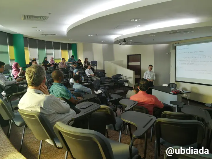
Soldiers are expected to perform complex and demanding tasks during operations, often while carrying a heavy load. It is therefore important for commanders to understand the relationship between load carriage and soldiers’ performance, as such knowledge helps inform decision-making on training policies, operational doctrines, and future soldier systems requirements. In order to investigate this, repeated experiments were conducted to capture key soldier performance parameters under controlled conditions. The data collected was found to contain missing values due to dropouts as well as non-measurement. We propose a Bayesian structural equation model to quantify a latent variable representing soldiers’ abilities, while taking into consideration the non-random nature of the dropouts and time-varying effects. This talk describes the modelling exercise conducted, emphasising the statistical model-building process as well as the practical reporting of the outputs of the model.
Links
References
- Bollen, K. A. (1989). Structural Equations with Latent Variables. John Wiley & Sons. ISBN: 978-0-471-01171-2. DOI: 10.1002/9781118619179.
- Denwood, M. (2016). runjags: An R Package Providing Interface Utilities, Model Templates, Parallel Computing Methods and Additional Distributions for MCMC Models in JAGS. Journal of Statistical Software 71.9, pp. 1–25. DOI: 10.18637/jss.v071.i09.
- Edwards, J. R. and R. P. Bagozzi (2000). On the nature and direction of relationships between constructs and measures. Psychological methods 5.2, p. 155.
- Hafez, M. S., I. Moustaki, and J. Kuha (2015). Analysis of multivariate longitudinal data subject to nonrandom dropout. Structural Equation Modeling: A Multidisciplinary Journal 22.2, pp. 193–201.
- Kruschke, J. K. (2014). Doing Bayesian Data Analysis: A tutorial with R, JAGS, and Stan. Second Edition. Boston: Academic Press. ISBN: 978-0-12-405888-0.
- Rabe-Hesketh, S. and A. Skrondal (2008). Multilevel and longitudinal modeling using Stata. STATA press.
Sample code in JAGS
model{
  for (i in 1:N) {
    for (k in 1:p_phy) {  # Physical
      y_phy[i,k] ~ dnorm(a_phy[k] + b_phy[k] * Phy[i], 1/v_phy[k])
    }
    for (k in 1:p_cgn) {  # Cognitive
      y_cgn[i,k] ~ dnorm(a_cgn[k] + b_cgn[k] * Cgn[i], 1/v_cgn[k])
    }
    for (k in 1:p_cmb) {  # Combatant
      y_cmb[i,k] ~ dnorm(a_cmb[k] + b_cmb[k] * Cmb[i], 1/v_cmb[k])
    }

    Phy[i] ~ dnorm(a_Phy + b_Phy * Abl[i], 1/v_Phy)
    Cgn[i] ~ dnorm(a_Cgn + b_Cgn * Abl[i], 1/v_Cgn)
    Cmb[i] ~ dnorm(a_Cmb + b_Cmb * Abl[i], 1/v_Cmb)

    Abl[i] ~ dnorm(a_Abl, 1/v_Abl)
  }

  # Priors ---------------------------------------------------------------------
  a_phy[1] ~ dnorm(0,1e-3)
  b_phy[1] <- 1
  for(k in 2:p_phy) {
    a_phy[k] ~ dnorm(0,1e-3)
    b_phy[k] ~ dnorm(0,1e-2)
  }
  for(k in 1:p_phy) {
    sd_phy[k] ~ dgamma(1,.5)
    v_phy[k]  <- pow(sd_phy[k],2)
  }

  a_cgn[1] ~ dnorm(0,1e-3)
  b_cgn[1] <- 1
  for(k in 2:p_cgn) {
    a_cgn[k] ~ dnorm(0,1e-3)
    b_cgn[k] ~ dnorm(0,1e-2)
  }
  for(k in 1:p_cgn) {
    sd_cgn[k] ~ dgamma(1,.5)
    v_cgn[k]  <- pow(sd_cgn[k],2)
  }

  a_cmb[1] ~ dnorm(0,1e-3)
  b_cmb[1] <- 1
  for(k in 2:p_cmb) {
    a_cmb[k] ~ dnorm(0,1e-3)
    b_cmb[k] ~ dnorm(0,1e-2)
  }
  for(k in 1:p_cmb) {
    sd_cmb[k] ~ dgamma(1,.5)
    v_cmb[k]  <- pow(sd_cmb[k],2)
  }

  a_Phy <- 0
  a_Cgn <- 0
  a_Cmb <- 0
  a_Abl <- 0

  b_Phy <- 1
  b_Cgn ~ dnorm(0,1e-2)
  b_Cmb ~ dnorm(0,1e-2)

  sd_Phy ~ dgamma(1,.5)
  v_Phy <- pow(sd_Phy,2)
  sd_Cgn ~ dgamma(1,.5)
  v_Cgn <- pow(sd_Cgn,2)
  sd_Cmb ~ dgamma(1,.5)
  v_Cmb <- pow(sd_Cmb,2)
  sd_Abl ~ dgamma(1,.5)
  v_Abl <- pow(sd_Abl,2)
}