Spatio-temporal modelling of property prices in Brunei Darussalam

LSE Social Statistics Seminar

Haziq Jamil

Assistant Professor of Statistics
Universiti Brunei Darussalam

https://haziqj.ml/lse-rms-oct23/

October 26, 2023

Table of contents

• Introduction
• Spatio-temporal models
• Application to Brunei data
• Next steps
• END

The team

Statistical modelling of spatio-temporal data in Brunei Darussalam

Motivation

Residential property price index (RPPI)

RPPI measures the rate at which the prices of private residential properties purchased by households are changing over time — BDCB

Ideally, any such index should capture the underlying trend in property values, rather than changes in characteristics of the houses being transacted.

Motivation

Methodological challenges

Hedonic regression is commonly employed to measure the constant-quality property price changes, i.e. \[ y_i = f(x_i, t_i) + \epsilon_i. \]

Some challenges faced:

• Data sparsity (infrequent transactions and missing covariates)
• Spatial and temporal autocorrelation
• Coverage and sample selection bias
• Data collection and processing

• Heterogeneity in property characteristics
  • e.g. land area, number of bedrooms, etc.
• Coverage geographical national vs cities, type of houses, cash/loan term
• Price (asking vs transacted vs appraised)
• Quality-mix adjustment (“bag of goods”) needs weighting. Essentially what is an “average house”?
• Timeliness of data, reliability, longevity, etc.

Motivation

Pretty visualisations

Source: github.com/Pecners

Introduction

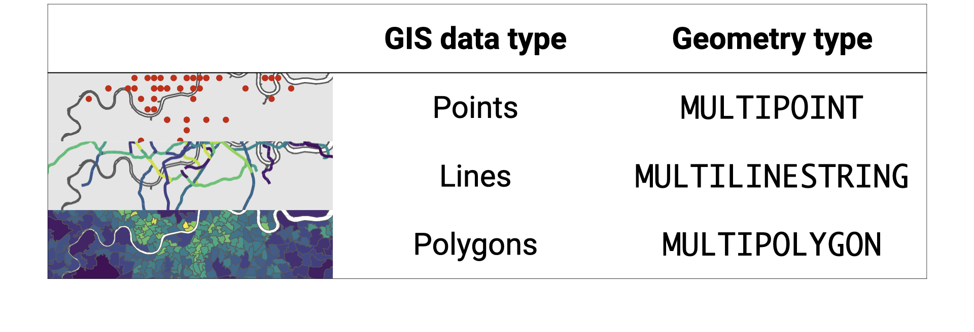
Types of spatial data

• Points
• Lines
• Polygons
• Others

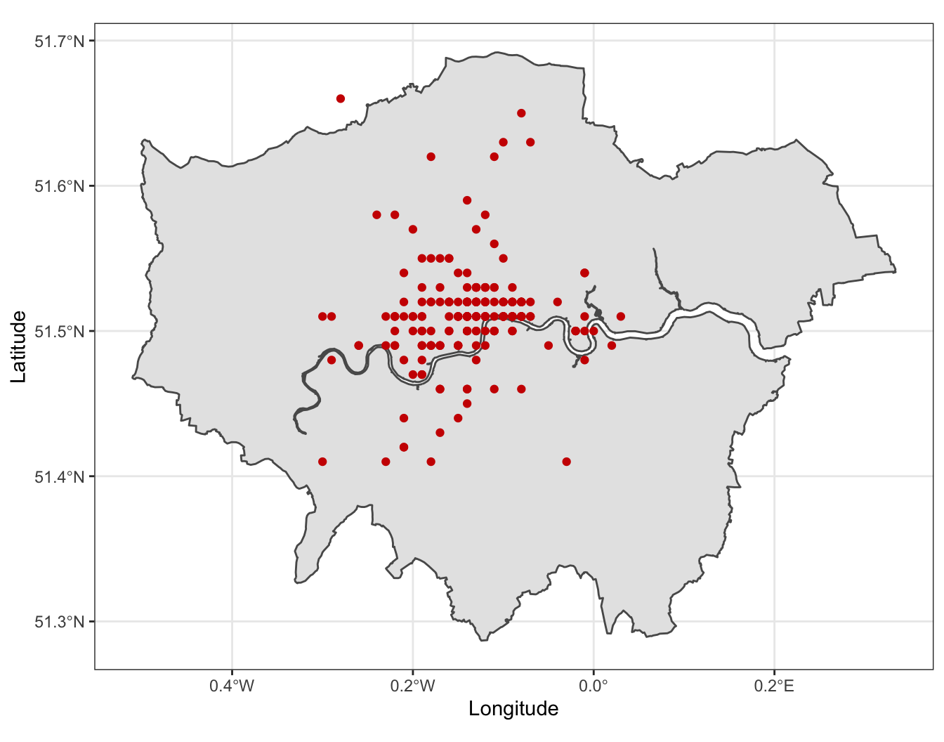
Location of Starbucks® around London.

Data source: Kaggle

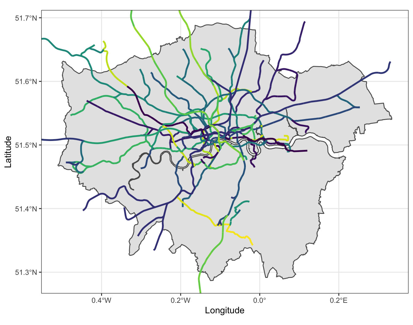
Transport for London (TFL) Tube, Overground, Elizabeth line, DLR & Tram lines (including Crossrail alignment)

Data source: github/oobrien

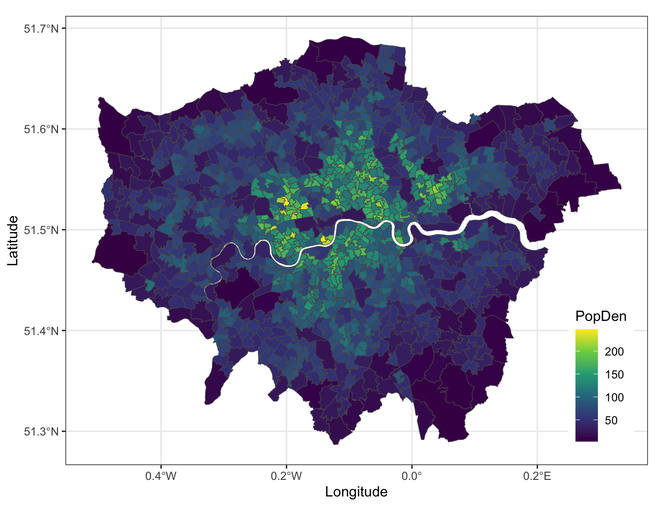
London Middle Super Output Area (MSOA) population density (2011).

Data source: London Datastore

• Geospatial points vs point processes
  • Point processes: Locations are random variables (e.g. earthquakes, crime, diseases, etc.)
  • Geospatial points: Locations are fixed
• Raster/Grid data
  • Pixelated (or gridded) data where each pixel is associated with a specific geographical location
  • E.g. satellite imagery, digital elevation models, etc.
• Network data.
  • E.g. road networks, social networks, etc.

Spatial data in R

• Simple features refers to a formal standard (ISO 19125-1:2004) that describes how objects in the real world can be represented in computers, with emphasis on the spatial geometry of these objects.
• The {sf} package (Pebesma and Bivand 2023) provides support for handling spatial data in R.

R has well-supported classes for storing spatial data (sp) and interfacing to the above mentioned environments (rgdal, rgeos), but has so far lacked a complete implementation of simple features, making conversions at times convoluted, inefficient or incomplete. The package sf tries to fill this gap, and aims at succeeding sp in the long term.

The standard is widely implemented in spatial databases (such as PostGIS), commercial GIS (e.g., ESRI ArcGIS) and forms the vector data basis for libraries such as GDAL. A subset of simple features forms the GeoJSON standard.

Spatial data in R (cont.)

london_sf |>  # read in using sf::st_read()
  select(MSOA11CD, LAD11NM, PopDen)

Simple feature collection with 983 features and 3 fields
Geometry type: MULTIPOLYGON
Dimension:     XY
Bounding box:  xmin: -0.5102995 ymin: 51.28676 xmax: 0.3339955 ymax: 51.69187
Geodetic CRS:  WGS 84
# A tibble: 983 × 4
   MSOA11CD  LAD11NM              PopDen                                geometry
   <chr>     <chr>                 <dbl>                      <MULTIPOLYGON [°]>
 1 E02000001 City of London         25.5 (((-0.0977199 51.52292, -0.097492 51.5…
 2 E02000002 Barking and Dagenham   31.3 (((0.1475682 51.59681, 0.1481361 51.59…
 3 E02000003 Barking and Dagenham   46.9 (((0.1510245 51.58589, 0.1510833 51.58…
 4 E02000004 Barking and Dagenham   24.8 (((0.1851372 51.56552, 0.1833498 51.56…
 5 E02000005 Barking and Dagenham   72.1 (((0.1492369 51.56738, 0.1483768 51.56…
 6 E02000007 Barking and Dagenham   50.6 (((0.1561951 51.56508, 0.1543864 51.56…
 7 E02000008 Barking and Dagenham   81.5 (((0.1357881 51.55903, 0.1344422 51.55…
 8 E02000009 Barking and Dagenham   87.4 (((0.1162061 51.557, 0.113344 51.55732…
 9 E02000010 Barking and Dagenham   76.8 (((0.1563492 51.55102, 0.1525812 51.55…
10 E02000011 Barking and Dagenham   38.8 (((0.1646052 51.55265, 0.1640759 51.55…
# ℹ 973 more rows

• E.g. Data set with (\(n=983\)) features containing spatial attributes (geometry) and feature-related variables (MSOA11CD, LAD11NM, PopDen).

• Notice the use of {dplyr} verbs! Link: Tidyverse methods for sf objects

Spatial analysis

To assess – or at least, to account – for spatial patterns in the data.

• Crucial to acknowledge the inherent non-randomness and interdependence within spatial data, increasing the validity and accuracy.

• Numerous motivations for doing so including

  • Agriculture (Besag and Higdon 1999)
  • Ecology (Brewer and Nolan 2007)
  • Education (Wall 2004)
  • Epidemiology (Xie et al. 2017; Li et al. 2011)
  • Image analysis (Gavin and Jennison 1997)

• Spatial statistics are indispensable for capturing the complexity of spatial data, leading to more accurate, reliable, and nuanced insights and decisions.

• Melanie Wall: To provide an example of this type of ecological spatial regression using these models we consider state level summary data related to the SAT college entrance exam for the year 1999.

• Spatial GAM to include X, Y coordinates for better disease mapping.

• Athma exacerbation and proximity of residence to major roads in Detroit, Michigan.

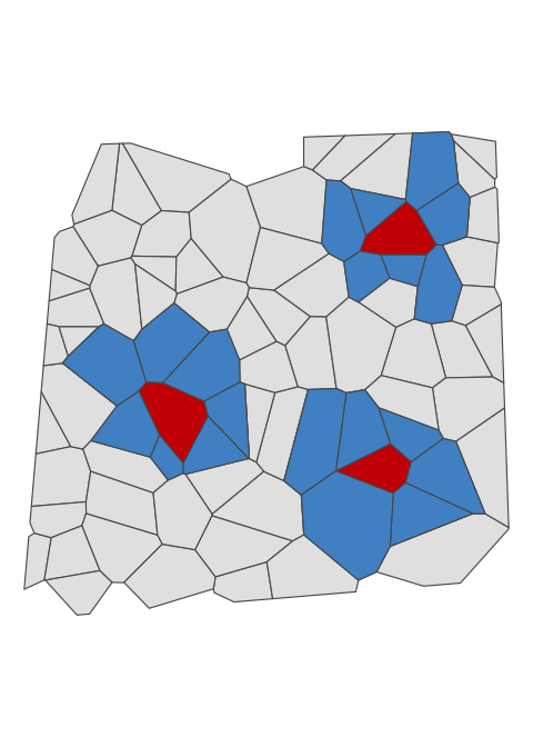
Types of spatial patterns

• Zero autocorrelation
• Positive autocorrelation
• Negative autocorrelation

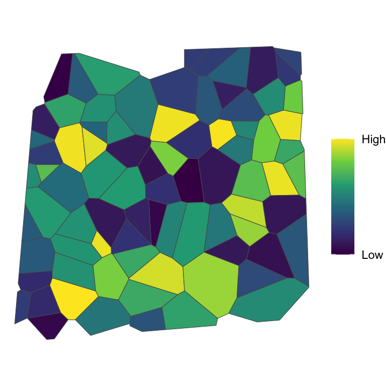
• Values are randomly distributed in space, independently of each other (and particularly its neighbours)

• Lack of a spatial pattern.

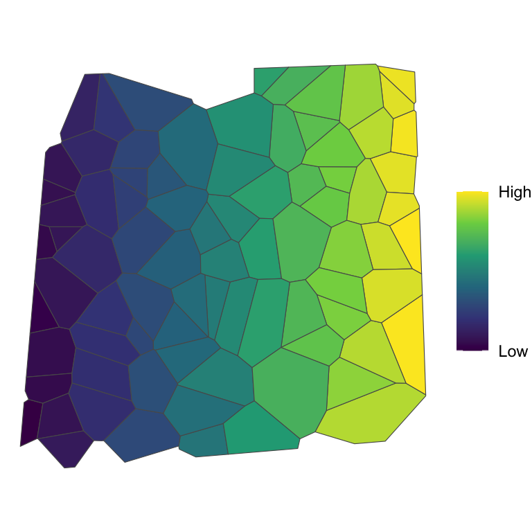
• Values are non-randomly distributed in space.

• Large values are “attracting” other large values, and vice versa.

• A clustering effect is present.

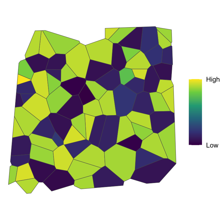
• Values are non-randomly distributed in space.

• Large values are “repelling” other large values, and vice versa.

• A dispersion effect is present.

Statistical test

Moran’s I test

• A test of “global” trends: Looks for evidence of spatial heterogeneity across the entire study area indexed by \(i=1,\dots,M\).

• The Moran’s I test statistic (1948) is defined as: \[ I = \frac{M}{\sum_{i}{\sum_{j}{w_{ij}}}} \frac{\sum_{i}{\sum_{j}{w_{ij}(y_i - \bar{y})(y_j - \bar{y})}}}{\sum_{i}{(y_i - \bar{y})^2}} \in [-1, 1] \] where \(w_{ij}\) is the “spatial weight” between locations \(i\) and \(j\).

• The null hypothesis is “the data are randomly distributed in space (no spatial autocorrelation)”, and is typically compared against an alternative of “>”.

• The Moran’s I value can be thought of as the ratio between the observed spatial variability and the expected variability.

Statistical test

Moran’s I test (cont.)

Two common approaches for \(p\)-value calculation:

\(Z\)-test

• Under \(H_0\), \(\operatorname{E}(I) = -1/(M-1)\).
• The variance \(\operatorname{Var}(I)\) also has a closed form expression.
• So, the CLT is invoked and a \(p\)-values based on a \(Z\) score is calculated.
• In practice, the normality assumption is not always met.

Permutation test

• Under \(H_0\), the spatial pattern is random, so we can shuffle the values and recompute \(I\).

• Compute the proportion of times \(I\) is larger than the observed value.

• The Monte Carlo approach can be more accurate.

Neighbour definitions

• A common approach is to give a weight of 1 if two zones are neighbors, and 0 otherwise

• Another common approach might be to give a weight of 1 to k nearest neighbors, 0 otherwise

• An alternative is to use a distance decay function for assigning weights.

• Sometimes the length of a shared edge is used for assigning different weights to neighbors

• The selection of spatial weights matrix should be guided by theory about the phenomenon in question. The value of I is quite sensitive to the weights and can influence the conclusions you make about a phenomenon, especially when using distances.

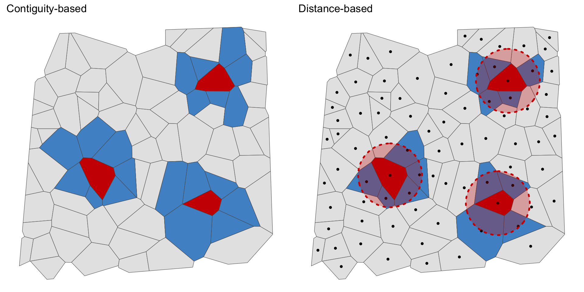
Adjacency matrix

For areal data it is quite common to implement \(W=A\) where \(A = (a_{ij})\) is an adjacency matrix with the following definition: \[ a_{ij} = \begin{cases} 1 & i \sim j \text{ where } i \neq j \\ 0 & \text{otherwise.} \end{cases} \]

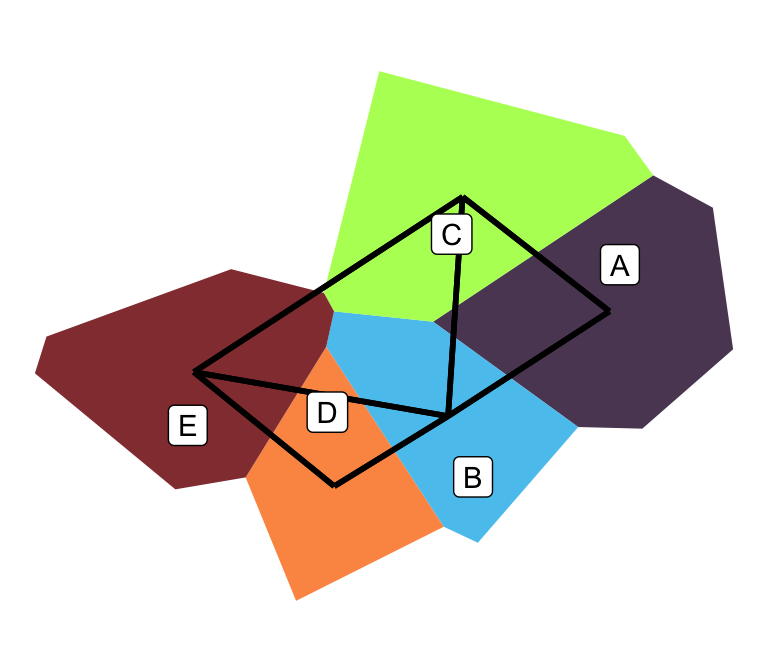
  A B C D E
A 0 1 1 0 0
B 1 0 1 1 1
C 1 1 0 0 1
D 0 1 0 0 1
E 0 1 1 1 0

Other useful definitions:

• \(D = \operatorname{diag}(A1)\) is a diagonal matrix containing number of neighbours.

• \(\tilde W = D^{-1}A\) is the scaled adjacency matrix (row sums are 1).

Example in R

library(spdep)
y <- negfc_sf$value
Wl <- poly2nb(negfc_sf) |> nb2listw(style = "B")
moran.test(y, listw = Wl, alternative = "less")

    Moran I test under randomisation

data:  y  
weights: Wl    

Moran I statistic standard deviate = -1.4695, p-value = 0.07084
alternative hypothesis: less
sample estimates:
Moran I statistic       Expectation          Variance 
      -0.11145491       -0.01234568        0.00454854 

moran.mc(y, listw = Wl, nsim = 1000, alternative = "less")

    Monte-Carlo simulation of Moran I

data:  y 
weights: Wl  
number of simulations + 1: 1001 

statistic = -0.11145, observed rank = 58, p-value = 0.05794
alternative hypothesis: less

Spatio-temporal models

Spatial areal unit models

The study area \(\mathcal S\) is partitioned into \(M\) non-overlapping areal units. To each areal unit \(i\) is associated a response variable \(y_i\) and a vector of covariates \(x_i\). Let \[ \begin{gather} y_i \sim p(y_i \mid \mu_i, \nu^2) \\ g(\mu_i) = x_i^\top\beta + \psi_i. \end{gather} \]

• Parameters of interest are \(\beta\) (regression coefficients) and \(\nu^2\) (response variance).

• \(g(\cdot)\) is a link function, e.g.

  • \(y_i \sim \operatorname{N}(\mu_i, \nu^2) \Leftrightarrow g(x) = x\)
  • \(y_i \sim \operatorname{Bin}(n_i, \pi_i) \Leftrightarrow g(x) = \log(\frac{x}{1-x})\)
  • \(y_i \sim \operatorname{Pois}(\mu_i) \Leftrightarrow g(x) = \log(x)\)

• Additionally, \(\psi_i\) are structured random effects to be estimated. It partly contains spatial random effects which we label \(\phi_i\).

Conditionally autoregressive (CAR) priors

Let \(\psi_i=\phi_i\). Then, the CAR prior (Leroux, Lei, and Breslow 2000) is defined as \[ \phi_i \mid \phi_{-i},W,\rho,\tau^2 \sim \operatorname{N}\left(\frac{\rho\sum_{j} w_{ij} \phi_j}{\rho\sum_{j} w_{ij}+1-\rho}, \frac{\tau^2}{\rho\sum_{j} w_{ij}+1-\rho}\right), \] where \(\rho\in[0,1]\) is a spatial dependence parameter; \(\tau^2\) is a variance parameter; and \(W\) is a known weight matrix (e.g. \(W=A \in \{0,1\}^{M\times M}\) adjacency matrix).

Special cases:

1. \(\rho = 0\) corresponds to independence;
2. \(\rho = 1\) corresponds to the Intrinsic CAR;
3. \(\rho=1\) and \(\psi_i = \phi_i + \theta_i\), where \(\theta_i\sim\operatorname{N}(0,\sigma^2)\) – this is the BYM (1991) model for binomial, Poisson and ZIP likelihoods.

CAR joint distribution

Using Brook’s lemma, the joint distribution of \(\phi\) (Besag 1974) is \[ (\phi_1,\dots,\phi_M)^\top \sim \operatorname{N}_M(0,\tau^2 Q^{-1}), \] where \[ Q = \rho[\overbrace{\operatorname{diag}(A1)}^{D}-\overbrace{A}^{DD^{-1}A}] + (1-\rho)I_M. \]

• Clearly \(Q\) is a convex combination of a fully intrinsic spatial structure \(Q=D(I_M - \tilde W)\) and a completely independent structure \(Q=I_M\).

• Estimating \(\rho\) from the data allows us to quantify the extent of spatial autocorrelation.

the “intrinsic” aspect of the ICAR model underscores the idea that the spatial effects it estimates are internally referenced and interconnected — they’re about the push and pull between areas, rather than independent, absolute measures. The model captures the fabric of spatial relationships, woven together through the constraints imposed on the estimates.

Aside

Simultaneously autoregressive models

In econometrics (LeSage and Pace 2009), the simultaneous autoregressive (SAR) model is more widely used: \[ \begin{gathered} y = \rho W y + X\beta + \epsilon \\ \epsilon \sim N_M(0, \sigma^2 I_M) \end{gathered} \]

• A direct spatial relationship between the response variables.

• Assume spatial interactions have a global effect (impacts are spread throughout the entire network of relationships).

• The \(\rho\) parameter is interpeted as the “spillover” effect.

• More appropriate to model “directional flow” by customising the \(W\) matrix.

Aside

Simultaneously autoregressive models

Adding the temporal element

Now suppose data at each spatial unit is recorded for \(t=1,\dots,T\) time periods. Extend the model: \[ \begin{gather} y_{it} \sim p(y_{it} \mid \mu_{it}, \nu^2) \\ g(\mu_{it}) = x_{it}^\top\beta + \psi_{it}. \end{gather} \]

We’ll discuss three ways to model the temporal dependence:

1. Linear time effects
2. ANOVA decomposition
3. Time autoregressive process

Adding the temporal element

Linear time effects (Bernardinelli et al. 1995)

Estimate the linear time trends for each areal unit. The goal is to estimate areas exhibiting changing linear trends in \(y\) over time. \[ \begin{gather} \psi_{it} = \phi_i + (\alpha + \delta_i)t \\ \phi_i \mid \phi_{-i} \sim \operatorname{CAR}(W, \rho, \tau^2) \\ \delta_i \mid \delta_{-i} \sim \operatorname{CAR}(W, \tilde\rho, \tilde\tau^2) \end{gather} \]

• Spatially varying intercept \(\phi_i\).
• Spatially varying time slope \(\alpha + \delta_i\), where \(\alpha\) is a “global” time effect.
• Assume linear temporal trend (like growth models).

Adding the temporal element

ANOVA decomposition (Knorr-Held 2000)

Decomposes the spatio-temporal variation into their constituent parts. The goal is to estimate overall time trends and spatial patterns. \[ \begin{gather} \psi_{it} = \phi_i + \delta_t + \gamma_{it} \\ \phi_i \mid \phi_{-i} \sim \operatorname{CAR}(W, \rho, \tau^2) \\ \delta_i \mid \delta_{-i} \sim \operatorname{CAR}(D, \tilde\rho, \tilde\tau^2) \\ \gamma_{it} \sim \operatorname{N}(0, \omega^2) \end{gather} \]

• \(\phi\) are the spatial random effects, and \(\delta\) are the temporal random effects.
• \(D\) is the “temporal adjacency” matrix: \(D_{tt'}=1\) if \(|t-t'|=1\), otherwise 0.
• The (optional) interaction terms \(\gamma_{it}\) are not identified for normal models.

Adding the temporal element

Time autoregressive process (Rushworth, Lee, and Mitchell 2014)

Include and AR(1) or AR(2) temporal process. The goal is to estimate the evolution of spatial random effects over time. \[ \begin{gather} \psi_{it} = \phi_{it} \\ \phi^{(t)} \mid \phi^{(t-1)},\phi^{(t-2)} \sim \operatorname{N}_M\big(a_1\phi^{(t-1)} + a_2\phi^{(t-2)}, \tau^2 Q(W,\rho)^{-1}\big) \hspace{2em} t\geq 3 \\ \phi^{(1)} \sim \operatorname{N}_M\big(0, \tau^2 Q(W,\rho)^{-1}\big) \end{gather} \]

• The \(Q\) precision matrix is the same as the CAR Leroux model.
• Temporal autocorrelation is induced by the mean.
• Spatial autocorrelation is induced by the variance.

Model estimation and inference

• Model estimated fully Bayesian using Markov chain Monte Carlo (MCMC) methods. Additional priors:
  • \(\beta \sim \operatorname{N}(\mu_\beta,\Sigma_\beta)\). Default choice of mean 0 and very large independent variance.
  • \(\Gamma^{-1}(1,0.01)\) for variance parameters.
  • \(\operatorname{Unif}(-1,1)\) for the \(\rho\)s.

• Use the {CARBayesST} package (Lee, Rushworth, and Napier 2018).
  • Gibbs sampling for closed-form full conditionals (e.g. \(\beta\), \(\phi\), \(\tau^2\)).
  • Metropolis or Metropolis-Hastings for the rest.
  • Make use of sparsity of \(W\) (and \(D\)) to speed up computation.

• Model fit criteria: Log-likelihood; Deviance information criterion (DIC) (Spiegelhalter et al. 2002); and Watanabe-Akaike information criterion (WAIC) (Watanabe and Opper 2010).

Application to Brunei data

The data

• Loan information data pertaining to residential property purchases obtained from BDCB as reported from financial institutions (2015–2022).

• \(N=3,512\) sample points spread across \(T=32\) quarters containing:

  0. price: Property price in thousands of Brunei dollars
  1. type: Property type (Land, Detached, Semi-Detached, Terrace, Apartment)
  2. built_up: Built up area in 1,000 square feet
  3. beds: No. of beds
  4. baths: No. of baths
  5. land_type: Land type (Freehold, Leasehold, Strata)
  6. land_size: Lot area in acres

• Model: price ~ house_characteristics + st_effects + error (Gaussian errors, identity link).

Spatial distribution of prices

• Brunei is administratively divided into four districts with \(M=39\) mukims (sub-districts).

• Some mukims will not have any transactions due to:

  • Nature reserve areas
  • Government land
  • No residential properties

• The \(W\) matrix is the binary mukim relationship ignoring the non-observed areas.

Moran’s test \(I =0.427, p = 9e-04\)

Aggregating data and missing values

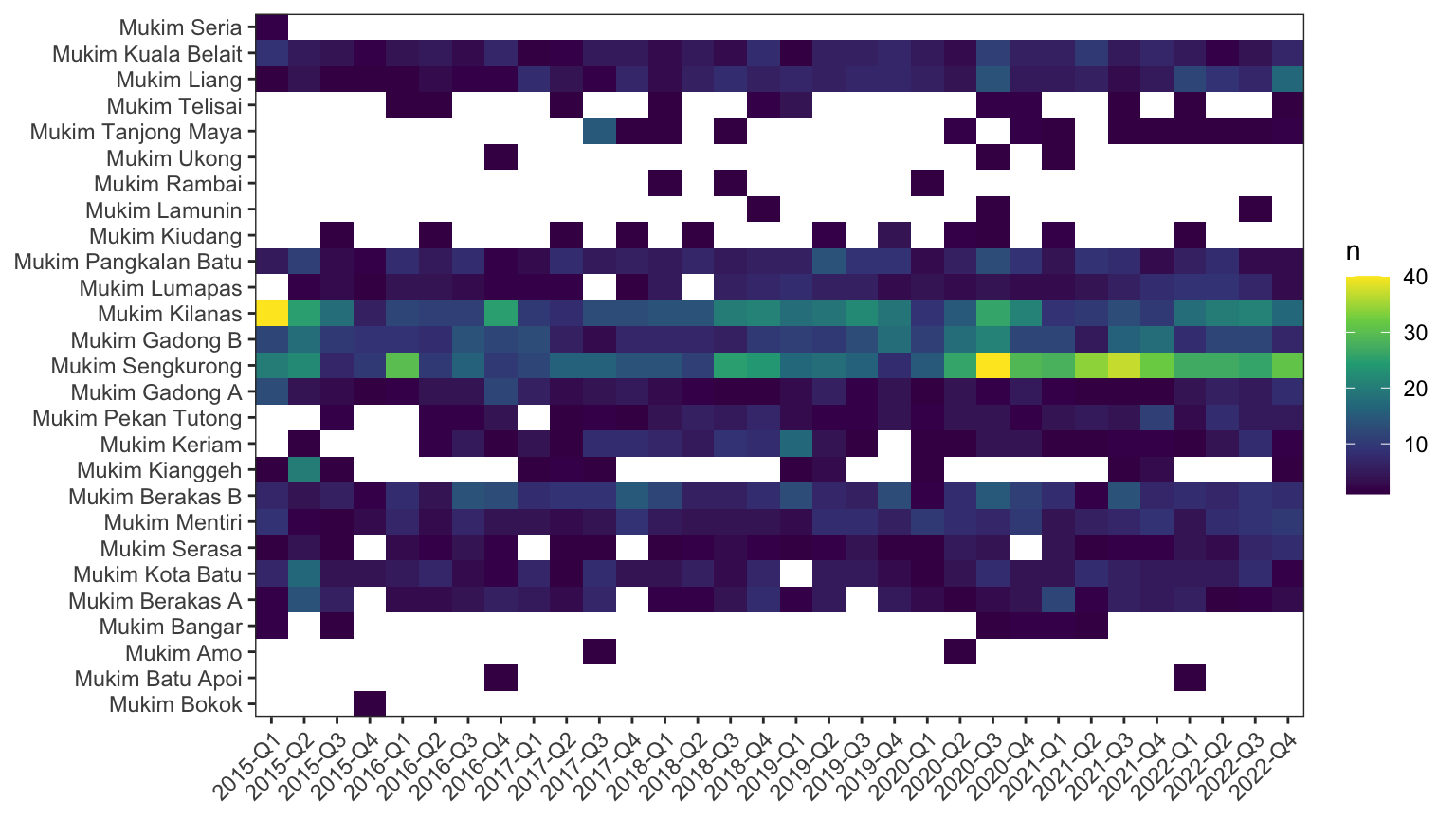
Spatio-temporal imputation

Everything is related to everything else, but near things are more related than distant things. — Tobler’s first law of geography

Strategy

1. For each \(i\), find its neighbours.
2. Subset data to \(i\)’s neighbours, and compute a 3-quarter rolling statistic
   • For continuous variables: the mean.
   • For discrete variable: the mode.
3. Repeat for 1–2 for each \(i\).
4. Repeat steps 1–3 using imputed data, until complete.

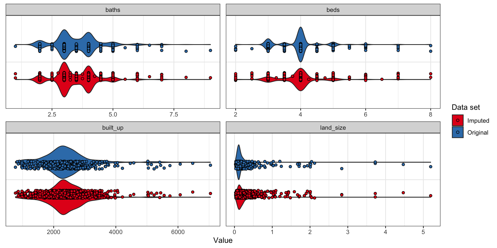
Validation of imputation method

Continuous variables

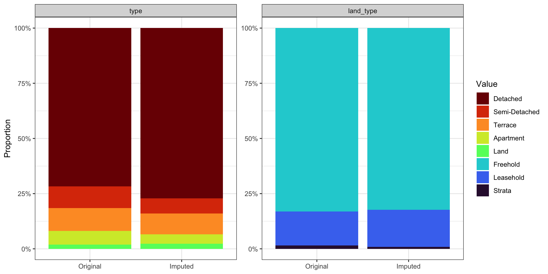
Validation of imputation method

Categorical variables

Model fit

	Base	Linear	ANOVA	AR(1)	AR(2)
Coefficients
(Intercept)	231 [172, 291] *	193 [145, 242] *	194 [146, 243] *	183 [135, 230] *	182 [135, 229] *
Type (ref: Land)
Detached	-150 [-219, -80.0] *	-114 [-171, -57.2] *	-113 [-171, -56.0] *	-87.3 [-144, -30.9] *	-87.9 [-144, -32.7] *
Semi-Detached	-147 [-218, -76.3] *	-126 [-185, -67.9] *	-127 [-186, -67.3] *	-96.3 [-155, -39.2] *	-96.5 [-154, -39.2] *
Terrace	-175 [-248, -102] *	-158 [-216, -99.1] *	-159 [-217, -100] *	-120 [-178, -61.4] *	-119 [-177, -61.8] *
Apartment	-55.5 [-125, 15.2]	-93.9 [-152, -36.9] *	-95.7 [-153, -39.1] *	-62.8 [-119, -5.76] *	-58.5 [-115, -2.36] *
Built up area (1000 sqft)	21.2 [9.07, 33.3] *	18.1 [8.78, 27.5] *	16.4 [7.22, 25.6] *	19.1 [10.2, 28.0] *	20.2 [11.2, 29.1] *
No. of beds	5.69 [-7.77, 19.3]	13.9 [3.21, 24.8] *	14.1 [3.19, 25.1] *	11.9 [1.27, 22.4] *	11.8 [1.29, 22.3] *
No. of baths	27.9 [16.5, 39.0] *	14.1 [5.08, 23.0] *	14.8 [5.79, 23.9] *	13.6 [4.82, 22.2] *	13.6 [4.85, 22.4] *
Land type (ref: Freehold)
Leasehold	18.3 [-3.02, 39.3]	6.26 [-15.2, 28.2]	6.41 [-15.0, 28.1]	3.44 [-16.7, 24.0]	3.39 [-17.2, 24.1]
Strata	71.5 [9.25, 134] *	30.4 [-19.8, 80.8]	31.6 [-19.1, 82.2]	6.56 [-41.6, 55.6]	2.46 [-46.3, 51.7]
Land area	-7.82 [-25.7, 10.1]	13.3 [-0.90, 27.5]	11.6 [-2.93, 26.1]	12.6 [-0.95, 26.4]	12.5 [-0.98, 26.2]
Spatio-temporal paramaters
rho.S		0.54 [0.12, 0.92] *	0.53 [0.11, 0.92] *	0.40 [0.11, 0.71] *	0.40 [0.12, 0.70] *
alpha		19.4 [0.36, 38.4] *
rho1.T		0.40 [0.02, 0.91] *	0.40 [0.02, 0.91] *	0.99 [0.96, 1.00] *	0.57 [0.30, 1.02] *
rho2.T					0.42 [-0.03, 0.69]
Variances
nu2	6514 [5761, 7362] *	3672 [3246, 4168] *	3693 [3261, 4177] *	2804 [2367, 3275] *	2524 [1954, 3103] *
tau2.S		9296 [4590, 17188] *	9214 [4562, 17204] *
tau2.T		2.01 [0.00, 0.09] *	0.02 [0.00, 0.09] *
tau2				718 [414, 1130] *	1477 [624, 2416] *
Model fit criterion
DIC	6137 (11.9)	5858 (36.0)	5861 (35.1)	5800 (120.6)	5782 (159.9)
WAIC	6151 (24.5)	5873 (46.1)	5876 (45.8)	5815 (113.8)	5802 (146.3)
LMPL	-3076	-2938	-2939	-2917	-2919
Loglik	-3056	-2893	-2895	-2779	-2731

Monopoly Brunei Edition

Monopoly Brunei Edition (cont.)

	mukim	phi	district
1	Mukim Kianggeh	220.38	Brunei Muara
2	Mukim Gadong A	113.11	Brunei Muara
3	Mukim Kuala Belait	89.68	Belait
4	Mukim Gadong B	70.08	Brunei Muara
5	Mukim Kota Batu	67.79	Brunei Muara
6	Mukim Berakas B	61.61	Brunei Muara
7	Mukim Berakas A	47.20	Brunei Muara
8	Mukim Sengkurong	40.73	Brunei Muara
9	Mukim Kilanas	34.72	Brunei Muara
10	Mukim Mentiri	33.88	Brunei Muara
11	Mukim Liang	25.05	Belait
12	Mukim Serasa	1.65	Brunei Muara
13	Mukim Seria	-4.34	Belait
14	Mukim Pangkalan Batu	-9.07	Brunei Muara

	mukim	phi	district
15	Mukim Lumapas	-11.83	Brunei Muara
16	Mukim Keriam	-16.52	Tutong
17	Mukim Telisai	-28.12	Tutong
18	Mukim Pekan Tutong	-34.55	Tutong
19	Mukim Bangar	-38.31	Temburong
20	Mukim Tanjong Maya	-39.93	Tutong
21	Mukim Kiudang	-71.02	Tutong
22	Mukim Lamunin	-71.51	Tutong
23	Mukim Ukong	-73.39	Tutong
24	Mukim Batu Apoi	-73.97	Temburong
25	Mukim Amo	-101.48	Temburong
26	Mukim Bokok	-113.37	Temburong
27	Mukim Rambai	-118.46	Tutong

Next steps

Multiple observations per area

• Areal data rely on aggregated observations. Lose the variability for the areal data point.

• Possible to extend the models “multilevel style”.

• Suppose we have \(j=1,\dots,M_i\) observations for each areal unit \(i\). Then (at least conceptually) \[ \begin{gather} y_{ijt} \sim p(y_{ijt} \mid \mu_{ijt}, \nu^2) \\ g(\mu_{ijt}) = x_{ijt}^\top\beta + \psi_{it}. \end{gather} \]

• Can we also extend this to the Moran’s I test?

Spatial imputation

• Need to study how best to handle the missing covariates.
• More sophisticated spatio-temporal imputation methods?
• Under a Bayesian paradigm, we could impute the missing covariates using the posterior predictive distribution.
• Graphical models.

RPPI-specific research

1. Need for time-varying regression coefficients?

   • It may not make sense that the coefficients are fixed for a long period of time.
   • Rolling window methods?

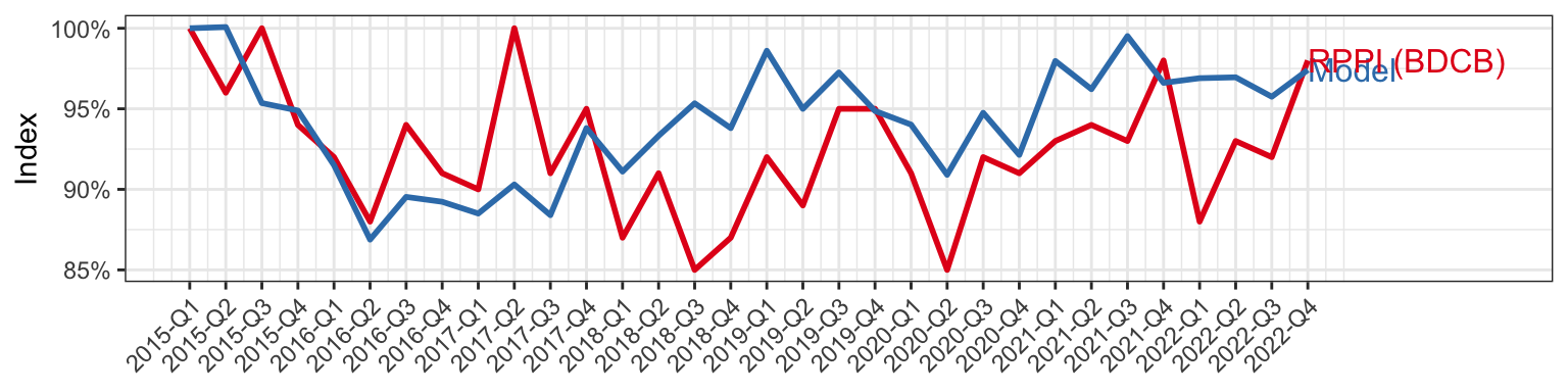
2. Building of RPPI by predicting price of an “average house” in quarter.

   • Mix adjustment methods? ‘Basket of goods’ analogy for building consumer price index.

3. Increasing coverage

   • Use advertised listings from real estate agents. Scrape online data.

END

Thanks!

References

Bernardinelli, Luisa, D Clayton, Cristiana Pascutto, Chiara Montomoli, Mauro Ghislandi, and Marco Songini. 1995. “Bayesian Analysis of Space—Time Variation in Disease Risk.” Statistics in Medicine 14 (21-22): 2433–43.

Besag, Julian. 1974. “Spatial Interaction and the Statistical Analysis of Lattice Systems.” Journal of the Royal Statistical Society: Series B (Methodological) 36 (2): 192–225.

Besag, Julian, and David Higdon. 1999. “Bayesian Analysis of Agricultural Field Experiments.” Journal of the Royal Statistical Society Series B: Statistical Methodology 61 (4): 691–746.

Besag, Julian, Jeremy York, and Annie Mollié. 1991. “Bayesian Image Restoration, with Two Applications in Spatial Statistics.” Annals of the Institute of Statistical Mathematics 43: 1–20.

Brewer, Mark J, and Andrew J Nolan. 2007. “Variable Smoothing in Bayesian Intrinsic Autoregressions.” Environmetrics: The Official Journal of the International Environmetrics Society 18 (8): 841–57.

Gavin, John, and Christopher Jennison. 1997. “A Subpixel Image Restoration Algorithm.” Journal of Computational and Graphical Statistics 6 (2): 182–201.

Knorr-Held, Leonhard. 2000. “Bayesian Modelling of Inseparable Space-Time Variation in Disease Risk.” Statistics in Medicine 19 (17-18): 2555–67.

Lee, Duncan, Alastair Rushworth, and Gary Napier. 2018. “Spatio-Temporal Areal Unit Modeling in r with Conditional Autoregressive Priors Using the CARBayesST Package.” Journal of Statistical Software 84: 1–39.

Leroux, Brian G, Xingye Lei, and Norman Breslow. 2000. “Estimation of Disease Rates in Small Areas: A New Mixed Model for Spatial Dependence.” In Statistical Models in Epidemiology, the Environment, and Clinical Trials, 179–91. Springer.

LeSage, James, and Robert Kelley Pace. 2009. Introduction to Spatial Econometrics. Chapman; Hall/CRC.

Li, Shi, Stuart Batterman, Elizabeth Wasilevich, Huda Elasaad, Robert Wahl, and Bhramar Mukherjee. 2011. “Asthma Exacerbation and Proximity of Residence to Major Roads: A Population-Based Matched Case-Control Study Among the Pediatric Medicaid Population in Detroit, Michigan.” Environmental Health 10 (1): 1–10.

Moran, Patrick AP. 1948. “The Interpretation of Statistical Maps.” Journal of the Royal Statistical Society. Series B (Methodological) 10 (2): 243–51.

Pebesma, Edzer, and Roger Bivand. 2023. Spatial Data Science: With applications in R. Chapman and Hall/CRC. https://doi.org/10.1201/9780429459016.

Rushworth, Alastair, Duncan Lee, and Richard Mitchell. 2014. “A Spatio-Temporal Model for Estimating the Long-Term Effects of Air Pollution on Respiratory Hospital Admissions in Greater London.” Spatial and Spatio-Temporal Epidemiology 10: 29–38.

Spiegelhalter, David J, Nicola G Best, Bradley P Carlin, and Angelika Van Der Linde. 2002. “Bayesian Measures of Model Complexity and Fit.” Journal of the Royal Statistical Society Series B: Statistical Methodology 64 (4): 583–639.

Wall, Melanie M. 2004. “A Close Look at the Spatial Structure Implied by the CAR and SAR Models.” Journal of Statistical Planning and Inference 121 (2): 311–24.

Watanabe, Sumio, and Manfred Opper. 2010. “Asymptotic Equivalence of Bayes Cross Validation and Widely Applicable Information Criterion in Singular Learning Theory.” Journal of Machine Learning Research 11 (12).

Xie, Sherrie, Rebecca Greenblatt, Michael Z Levy, and Blanca E Himes. 2017. “Enhancing Electronic Health Record Data with Geospatial Information.” AMIA Summits on Translational Science Proceedings 2017: 123.