Leveraging sparse Gaussian processes for property price modelling and sustainable urban planning

Please cite this work as:

Jamil, H., Usop, F., & Ramli, H. M. (2024). Leveraging Sparse Gaussian Processes for Property Price Modelling and Sustainable Urban Planning. In S. A. Abdul Karim & A. Baharum (Eds.), Intelligent Systems of Computing and Informatics in Sustainable Urban Development. Taylor and Francis/CRC Press.

@incollection{jamil2024foundation,
  title = {{{Leveraging Sparse Gaussian Processes}} for {{Property Price Modelling}} and {{Sustainable Urban Planning}}},
  booktitle = {Intelligent {{Systems}} of {{Computing}} and {{Informatics}} in {{Sustainable Urban Development}}},
  author = {Jamil, Haziq and Usop, Fatin and Ramli, Huda M.},
  editor = {Abdul Karim, Samsul Ariffin and Baharum, Aslina},
  year = {2024},
  series = {Intelligent {{Systems}} of {{Computing}} and {{Informatics}}},
  publisher = {{Taylor and Francis/CRC Press}}
}

1 Introduction

Sustainable urban planning plays a crucial role in shaping the global urban population by focusing on developing and managing cities in a way that encourages sustainability. With over half of the world’s population already living in urban areas, this number is expected to rise to 70 percent by 2050. The United Nations SDG 11 aims to create inclusive, safe, resilient, and sustainable cities and human settlements. This objective addresses various aspects of urban life and planning with the goal of enhancing the overall quality of life for city dwellers. Key focus areas include ensuring adequate housing and essential services, establishing sustainable transportation systems, preserving cultural and natural heritage, minimizing the negative environmental impact of cities, facilitating access to green spaces and public areas, as well as bolstering urban resilience against disasters (United Nations, 2018).

In order to effectively achieve the goals of sustainable urban planning, accurate and comprehensive models for analyzing property price evaluation are necessary. These models can inform urban planning decisions by predicting and assessing property prices, and guide in the shaping of inclusive and sustainable urban areas. They play a critical role in identifying affordable housing options, strategizing efficient transportation networks, distributing resources for infrastructure development, and promoting fair access to vital services (Dede, 2016) — all aligned with the UN SDG11 objectives. Statistical models are powerful tools in this regard, by providing insights into factors that influence property prices including location, amenities, infrastructure, and socioeconomic elements.

Scenario analysis stands as a valuable tool for evaluating the impact of different urban planning strategies by providing a structured framework to analyse and visualise different planning approaches, helping to inform and guide towards more sustainable urban development outcomes (Kropp & Lein, 2013). Through a combination of qualitative narratives and quantitative data modeling, scenario analysis facilitates better decision-making by bridging the gap between intricate urban dynamics and strategic planning. It empowers planners to consider the future thoroughly when developing sustainable environments. Here are three examples of how data modelling can be used to support sustainable urban planning:

1. Urban Planning and Development Efficiency: Data models could be applied to analyse how urban planning decisions affect housing prices over time and space. An example of this is the work by Johnson (2007). By modelling the spatial distribution and temporal changes in house prices, insight can be provided into which urban development strategies are most effective at promoting affordable housing. This could support policy-making in urban development that aims for equitable growth and sustainability.

2. Assessment of Infrastructure Impact: Study the impact of infrastructure developments (like new transportation lines, parks, or public facilities) on local real estate values using data models. This application could help city planners understand the economic effects of their infrastructure projects, guiding them in making investments that lead to more sustainable urban environments and enhanced community welfare. See for instance, Shrestha et al. (2022) or Schoeman (2019).

3. Environmental Sustainability Analysis: Data models could be used to explore the relationship between house prices and environmental factors, such as proximity to green spaces, pollution levels, and environmental risk factors (like flooding). This analysis can help identify how environmental sustainability is valued in urban real estate and guide the planning of greener, more resilient urban areas that align with SDG11’s objectives. Recent strides in this area has been made by Mironiuc et al. (2021) and Chuweni et al. (2024).

Many different data modelling approaches exist in machine learning and statistical modelling, but Gaussian Process (GPs) have emerged as a non-parametric approach to regression tasks, where it is widely used to make uncertainty predictions for unseen input locations. Unlike their parametric counterparts such as the widely used class of linear regression models, non-parametric models offer unparalleled flexibility by making fewer assumptions about the data’s underlying structure, which often results in enhanced predictive power for complex datasets. The ease-of-use of GPs, as well as its adaptability to wide-ranging datasets, are what makes it practical for various domains. The techniques itself does not limit itself for the use of statisticians only, but it is also well known among other professions where it is important to define uncertainty predictions, such as finance, health care, and geology¹. Despite its apparent advantages, GP regression faces difficulties due to its unfavorable computational demands for larger data sets. This includes challenges related to time complexity and storage. As a result, there have been numerous attempts to find more efficient methods that provide an approximation while still preserving the underlying structure of the full exact GP solution as best as possible.

In recent years, there have been many attempts to address this limitation with the use of a method called the sparse approximation, where ‘sparse’ refers to the smaller subset of the data set. The authors of Rasmussen & Williams (2006) tackled this challenge using the Nyström method, which uses a low-rank approximation technique on the \(n\times n\) kernel matrix. This involves selecting a representative sample of \(m\) points from the dataset (where \(m \ll n\)) to construct an approximation. The full kernel matrix is then projected onto the subspace formed by the kernel matrix of this subset in order to approximate it, significantly reducing computational complexity.

Significant strides in Sparse Gaussian Process (GP) methods have enhanced the scalability of GPs for handling large datasets and mostly build off the Nyström approximation method. Csató (2002) advanced an iterative sparse approximation method that incrementally selects the most informative basis functions, laying the foundation for subsequent developments in active learning strategies within the GP framework. Building on the concept of data summarization, Snelson & Ghahramani (2005) introduced the use of pseudo-inputs, optimizing these alongside the model’s hyperparameters to reduce computational complexity by focusing only on a subset of training data. Further refining the efficiency and accuracy of these methods, Titsias (2009) proposed a variational approach that optimizes the lower bound of the marginal likelihood with respect to inducing variables, enhancing the approximation of the GP posterior. Extending these methodologies to even larger datasets, Hensman et al. (2013). adapted the variational framework to incorporate stochastic variational inference, allowing GPs to be applied to datasets with millions of points and supporting complex models with non-Gaussian likelihoods and latent variables. Significantly, the methodologies developed by Hensman et al. (2013) are accessible to the wider community, as they have been implemented in the GPy library for Python, facilitating their use in practical applications. These cumulative efforts demonstrate a progression from foundational sparse techniques to sophisticated large-scale applications in the GP domain.

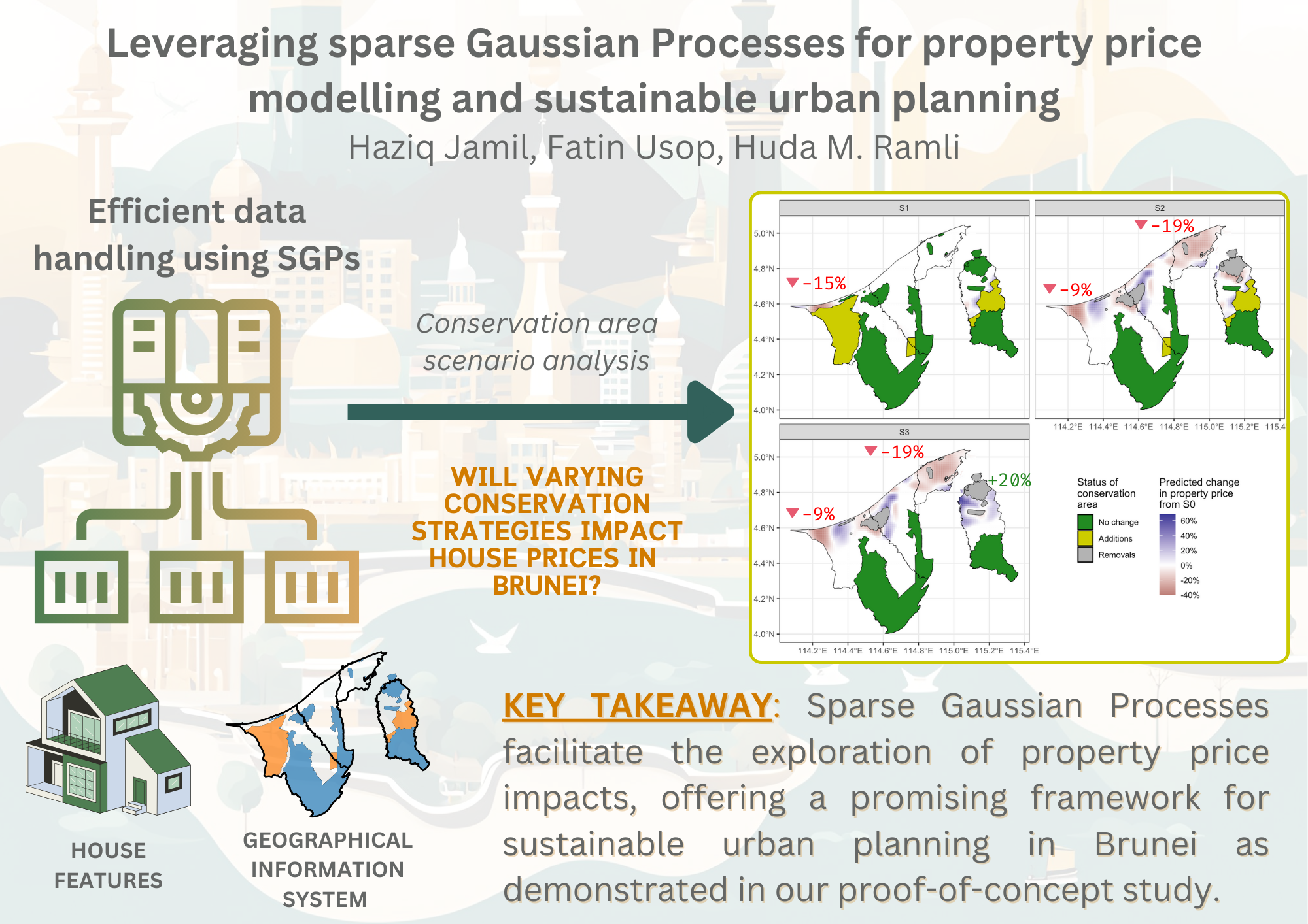
This paper aims to succinctly introduce the concept of Sparse Gaussian Processes from a soft mathematical standpoint, which include visualisation of the eveolution of the optimisation process using Python and R software, hopefully being instructive to the novice reader. As an application piece, we incorporate the principles of sustainable urban planning into property price modelling in Brunei Darussalam using sparse Gaussian Processes. The main interest is to evaluate the impact of different urban planning strategies on property prices, focusing on scenario analysis to inform sustainable urban development. This is inline with the broader objectives of creating inclusive, safe, and sustainable cities as outlined in the UN SDG 11.

2 Gaussian processes

For real-valued observations \(\mathbf{y} = (y_1,\dots,y_n)^\top\) and corresponding multivariate inputs \(x_1,\dots,x_n\), where each \(x_i\) belongs to a covariate set \(\mathcal{X}\), consider the regression problem represented by \[ y_i = f(x_i) + \epsilon_i, \quad i=1,\dots,n. \tag{1}\] The \(\epsilon_i\) terms are independent and identically distributed (iid) Gaussian noise terms with zero mean and variance \(\sigma^2\). Here, \(f\) is a regression function that we aim to estimate in order to make predictions and conduct inferences.

As the name implies, a Gaussian process (GP) essentially entails defining a Gaussian distribution over the random vector \(\mathbf{f} = \big(f(x_1),\dots,f(x_n) \big)^\top\) with mean \(\mathbf{m}\) and covariance matrix \(\mathbf{K}\). We may write \(\mathbf{f} \mid \mathcal{X} \sim \mathcal{N}(\mathbf{m},\mathbf{K})\), and refer to the probability density function of \(\mathbf{f}\) as \(p(\mathbf{f})\). The defining feature of the GP regression is the specification of a symmetric and positive-definite function \(k:\mathcal{X}\times\mathcal{X} \to \mathbb{R}\) known as the kernel function that determines the covariance \(\mathbf{K}_{ij}\) between the function values at any two input locations \(x_i\) and \(x_j\). Hence the GP is fully specified by the mean and kernel function, where conventionally the mean is set to zero a priori.

In many branches of mathematics, the kernel function is often viewed as a measure of similarity between the input locations. In the context of GP regression, similarity between input points \(x_i\) and \(x_j\) is reflected in the covariance \(\mathbf{K}_{ij}\), which in turn influences the similarity of the outputs \(f(x_i)\) and \(f(x_j)\). Different types of kernel functions can be used to affect different notions of similarity, and the choice of kernel is often crucial to the performance of the GP regression model. Examples of popular kernels include the squared exponential kernel and the Matérn kernel, as defined in Table 1.
The squared exponential kernel yields smoother and more continuous outputs, embodying an assumption of high regularity, whereas the Matérn kernel, with its additional flexibility in the smoothness parameter, is adept at modelling more abrupt and irregular changes in the data. The user must choose the kernel function that best captures the underlying structure of the data, and this choice is often guided by domain knowledge and the nature of the data.

Table 1: Explicit definitions for two popular kernels in GPR. For the Matérn kernel, \(K_\nu\) is the modified Bessel function of the second kind, and \(\Gamma(\cdot)\) is the gamma function.

Name	\(k(x,x')\)	Hyperparameters
Squared exponential	\[\lambda \exp\left(-\frac{\|x-x'\|^2}{2\ell^2}\right)\]	\(\ell\) lengthscale; \(\lambda\) amplitude
Matérn	\[\lambda \frac{2^{1-\nu}}{\Gamma(\nu)} \left(\frac{\sqrt{2\nu} \, d}{\ell}\right)^\nu K_\nu\left(\frac{\sqrt{2\nu} \, d}{\ell}\right)\]	\(\nu\) smoothness parameter; \(\ell\) lengthscale; \(\lambda\) amplitude

The GP on \(\mathbf{f}\) cab be thought of as a prior distribution over the space of regression functions in a Bayesian sense. Together with Equation 1, we may write \[ \mathbf{y} \sim \mathcal{N}(\mathbf{m},\mathbf{K} + \sigma^2\mathbf{I}), \tag{2}\] specifying a Gaussian likelihood for the observed data vector \(\mathbf{y}\). Hence, the GP is a conjugate prior for the regression function \(f\) in the presence of Gaussian noise. Specifically, we have that \(f \mid\mathbf{y}\sim\mathcal{N}\big(\hat m,\hat k \big)\), where the mean and covariance functions are given by \[ \begin{aligned} \hat m(x) &= \mathbf{K}(x)^\top\big(\mathbf{K} + \sigma^2\mathbf{I}\big)^{-1}\mathbf{y},\\ \hat k(x,x') &= k(x,x') - \mathbf{K}(x)^\top\big(\mathbf{K} + \sigma^2\mathbf{I}\big)^{-1}\mathbf{K}(x'), \end{aligned} \] for any \(x,x'\in\mathcal{X}\), where \(\mathbf{K}(x)=\big(k(x_1,x),\dots,k(x_n,x)\big)^\top\). This is a well known result in the GP literature – see e.g. Ishida & Bergsma (2023) for a detailed derivation. Clearly, the posterior distribution applies to any input \(x\) from the domain set \(\mathcal{X}\), including new input locations not present in the training data, allowing the GP to make predictions at arbitrary locations. Additionally, the posterior distribution is Gaussian, which facilitates the computation of credible intervals and point estimates for the regression function.

The kernels used may involve hyperparameters which may either be chosen by the user, or estimated from the data. In the latter case, the hyperparameters are typically estimated by maximizing the likelihood function of the data after marginalising out the GP prior given by Equation 2. Methods such as conjugate gradients are typically employed, with a Choleski decomposition on the kernel matrix \(\mathbf{K}\) to facilitate the computations (Rasmussen & Williams, 2006). Alternatively, quasi Newton methods such as L-BFGS-B may be used to optimise the hyperparameters, which are often more efficient for large data sets. Jamil & Bergsma (2019) employed an EM algorithm for a certain class of Gaussian priors known as I-priors.

Whether the hyperparameters are estimated or chosen by the user, calculation of the GP posterior involves the inversion of an \(n \times n\) kernel matrix. For very large data sets, this inversion can be computationally expensive both in time and storage, scaling to to the order of \(O(n^3)\) and \(O(n^2)\) respectively, prohibiting the use GP regression. In the next section, we discuss the use of sparse GPs as a solution to this problem.

3 Sparse Gaussian processes

Sparse Gaussian processes (SGPs) are a class of methods that aim to reduce the computational complexity of GP regression by approximating the full GP with a smaller set of inducing points. Suppose we have a set of \(m\) inducing points \(\mathbf{Z} = \{z_1,\dots,z_m\}\), where \(m \ll n\) and each \(z_i \in \mathcal{X}\) but not necessarily in the original training set. Denote by \(\mathbf{u} = (u_1,\dots,u_m)^\top\) the latent function values at the inducing points, i.e. \(u_i = f(z_i)\) for each \(i=1,\dots,m\). A priori, assume a GP prior over both \(\mathbf f\) and \(\mathbf u\): \[ \begin{pmatrix} \mathbf{f}\\ \mathbf{u} \end{pmatrix} \sim \mathcal{N} \left( \mathbf{0}, \begin{pmatrix} \mathbf{K} & \mathbf{K}_{uf}^\top\\ \mathbf{K}_{uf} & \mathbf{K}_u \end{pmatrix} \right) \] The quantities \(\mathbf{K}_{uf}\) and \(\mathbf{K}_u\) are the cross-covariance matrix between the function values at the inducing points and the original data points, and the covariance matrix of the function values at the inducing points respectively–both computed using the choice of the kernel function \(k(x,x')\). Note that we have used, for simplicity, a zero-valued mean function for the prior. Using standard results for the multivariate normal distribution, the conditional distribution of \(\mathbf{f}\) given \(\mathbf{u}\) is \[ \mathbf{f} \mid \mathbf{u} \sim \mathcal{N}\big(\mathbf{K}_{uf}\mathbf{K}_u^{-1}\mathbf{u},\mathbf{K} - \mathbf{Q} \big), \] where \(\mathbf{Q}=\mathbf{K}_{uf}\mathbf{K}_u^{-1}\mathbf{K}_{uf}^\top\) represents the reduction in the variance of \(\mathbf{f}\) due to the information from the inducing points \(\mathbf{u}\). Incidentally it is also referred to as the Nyström approximation of the kernel matrix \(\mathbf{K}\).

Ultimately the goal would be to compute the joint posterior \(p(\mathbf{f},\mathbf{u} \mid \mathbf{y})\), but evidently this is intractable for large \(n\), the same problem encountered in the previous section. To approximate the intractable true posterior, a variational distribution is introduced: \[ q(\mathbf{f},\mathbf{u}) = p(\mathbf{f} \mid \mathbf{u})q(\mathbf{u}), \] where \(q(\mathbf{u})\) is a variational approximation to the true posterior of the inducing variables, typically chosen to be a Gaussian distribution with its own variational parameters. Included in the variational parameters are the locations of the inducing points, since these highly determine the quality of the approximation. The variational parameters are then optimised to minimise the Kullback-Leibler (KL) divergence from the variational distribution to the true posterior.

As per Titsias (2009), the minimisation of this KL divergence is equivalent to maximising the so-called evidence lower bound (ELBO) \[ \mathcal{L}(\mathbf{Z}) = \log \phi(\mathbf{y} \mid \mathbf{0}, \mathbf{Q} + \sigma^2\mathbf{I}) - \frac{1}{2\sigma^2}\operatorname{tr}\big(\mathbf{K} - \mathbf{Q}\big) \] where \(\phi(\mathbf{y} \mid \boldsymbol{\mu},\boldsymbol{\Sigma})\) is the density function for \(\mathbf{y}\sim\mathcal{N}(\boldsymbol{\mu},\boldsymbol{\Sigma})\), and \(\mathbf{Q}\) is the Nyström approximation as previously defined. The optimal variational distribution, call this \(\tilde q\), is found to be a multivariate gaussian distribution over \(\mathbf{u}\) with mean and covariance given by \[ \begin{aligned} \boldsymbol{\mu}_u &= \sigma^{-2}\mathbf{K}_{u}\boldsymbol{\Psi}\mathbf{K}_{uf}\mathbf{y} \\ \boldsymbol{\Sigma}_u &= \mathbf{K}_u \boldsymbol{\Psi} \mathbf{K}_u \\ \boldsymbol{\Psi} &= (\mathbf{K}_u + \sigma^{-2}\mathbf{K}_{uf}\mathbf{K}_{uf}^\top\big)^{-1} \end{aligned} \] Evaluation of \(\tilde q\) requires hyperparameter values for the kernel, which can be optimised simultaneously with the variational parameters. The posterior distribution \(f\mid\mathbf{y}\) can then be obtained via \[ \begin{aligned} p(f \mid \mathbf{y}) &= \int p(f,\mathbf{u}\mid\mathbf{y}) \text{d} \mathbf{u} \\ &\approx \int p(f \mid \mathbf{u})\tilde q(\mathbf{u}) \text{d} \mathbf{u} \end{aligned} \] where the integral marginalises the inducing variables \(\mathbf{u}\) as a replacement for the true posterior distribution \(p(\mathbf{u} \mid \mathbf{y})\). This can be computed analytically as being Gaussian. Specifically, \(f \approx \mathbf{y}\sim\mathcal{N}\big(\tilde m,\tilde k \big)\), where the mean and covariance functions are given by \[ \begin{aligned} \tilde m(x) &= \sigma^{-2}\mathbf{K}_m(x)^\top\boldsymbol{\Psi}\mathbf{K}_{uf}\mathbf{y},\\ \tilde k(x,x') &= k(x,x') - \mathbf{K}_m(x)^\top\big(\mathbf{K}_u^{-1} - \boldsymbol{\Psi})\mathbf{K}_m(x'). \end{aligned} \] for any \(x,x'\in\mathcal{X}\), with \(\mathbf{K}_m(x)=\big(k(z_1,x),\dots,k(z_m,x)\big)^\top\) and \(\boldsymbol\Psi\) as defined above. The calculation of this approximate posterior avoids the need to invert any \(n\times n\) matrix, reducing the computational time complexity from \(O(n^3)\) to \(O(nm^2)\).

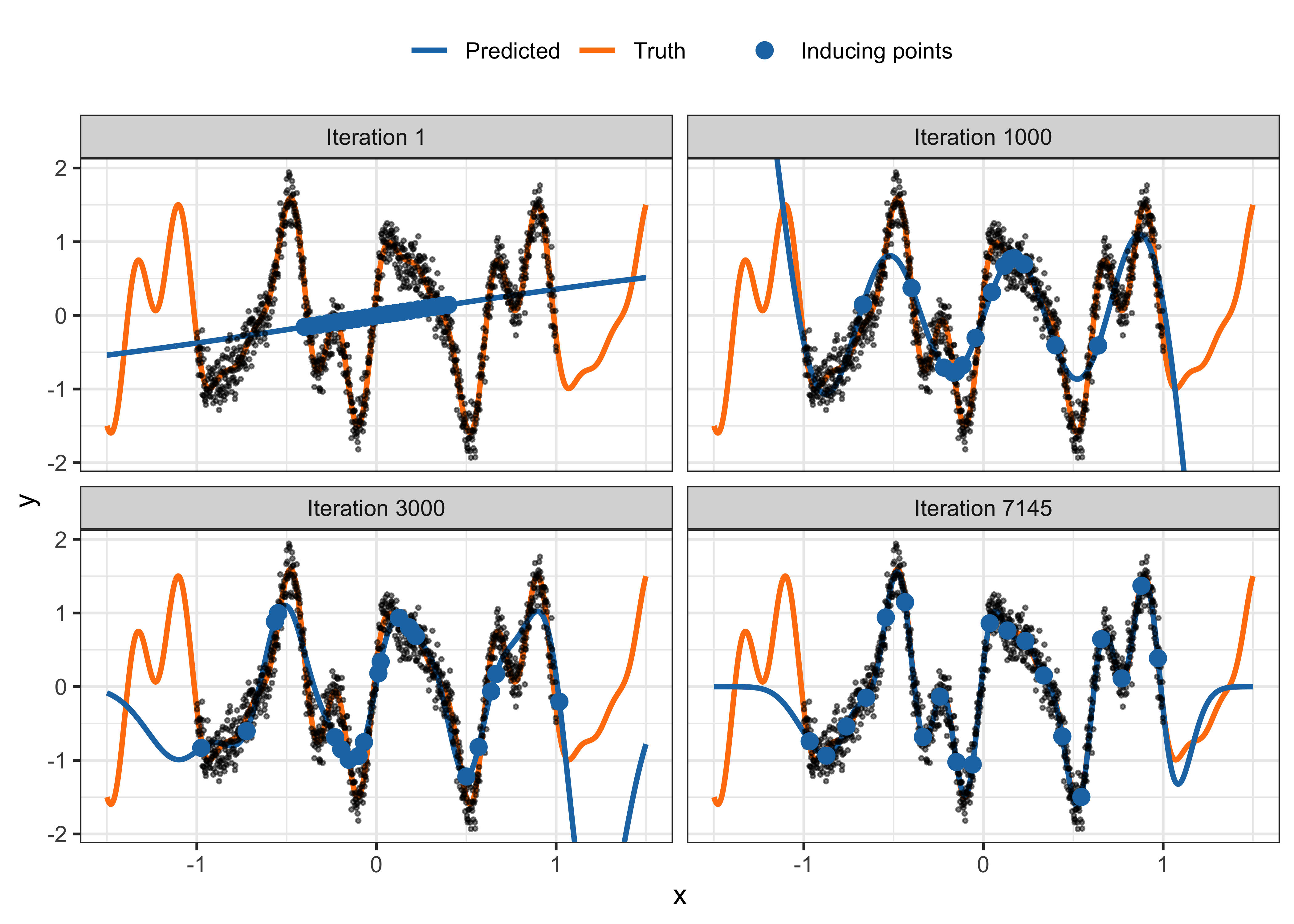
To illustrate the SGP method, consider obtaining \(n=1000\) noisy observations from the one-dimensional function taking one-dimension input \(x\in\mathbb{R}\). \[ f(x) = \sin(3\pi x) + 0.3\cos(9\pi x) + 0.5\sin(7\pi x). \] The variance \(\sigma^2\) of the noise is set to \(0.2\). This example was taken from documentation of GPflow (Matthews et al., 2017 – section on Stochastic Variational Inference for scalability with SVGP). A smooth RBF kernel is used to model the function, with \(m=50\) inducing points. The lengthscale and variance parameters of the kernel require optimising, along with the values of the inducing points \(z_1,\dots,z_m\). Good initial values will indeed help the optimisation process, but for illustration here we use \(m=50\) values equally spaced between -0.4 and 0.4. Figure 1 shows the evolution of the optimisation process, particularly the impact of the inducing points on the predicted regression function. At the start, the choice of equally spaced inducing points clearly gives a poor approximation to the true function. As the optimisation progresses, the inducing points are adjusted to better capture the function, leading to a more accurate prediction. The code for this example is made available in the supplementary material.

Figure 1: Evolution of the optimisation process and its impact on the predicted regression function.

4 Scenario analysis in urban planning

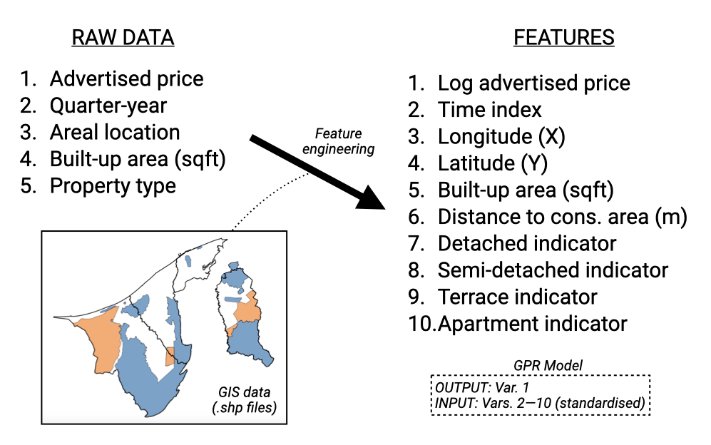
We showcase an application of using sparse GPs for scenario analysis in urban planning, with the running theme of sustainable development for cities and communities. The analysis focuses on modelling property prices in Brunei Darussalam, which is a small country in Southeast Asia located on the island of Borneo. Residential property data sourced from property listings from various real estate agents are available, including price, areal location, built up area (in square feet), the type of property (detached, semi-detached, terrace, or apartment) and date of listing (in quarter-years). The size of the dataset is \(n=11,351\) and it spans a period of 18 years, from 2006 to 2023. We note that missing values exist in the dataset, which were treated with a simple spatio-temporal mean imputation – see Jamil (2024) for details. The aim is to build a sparse GP model that can predict property prices sufficiently well across different regions in Brunei.

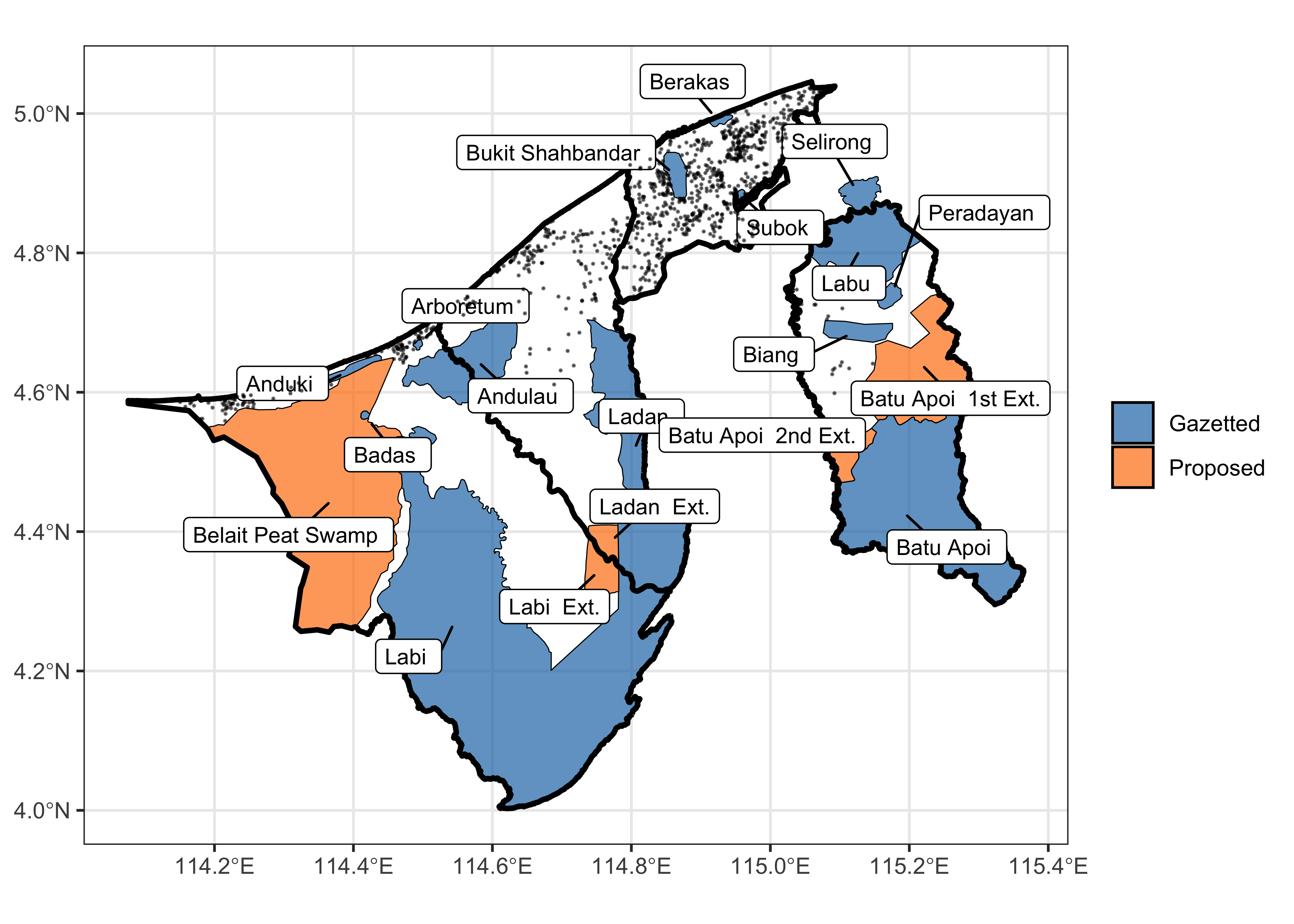
The report on the Convention on Biological Diversity in Brunei (Forestry Dept., 2014) highlights the nation’s commitment to preserving biodiversity through the establishment and maintenance of forest reserves. Specific areas have been officially designated as forest reserves, outlining both currently protected areas and plans for future gazettement to enhance environmental conservation efforts.

It is crucial for city planners to use scenario analysis to assess how various urban development strategies might influence property prices in Brunei. These scenarios focus on changes to forest reserve conservation efforts and their effects on nearby property values.

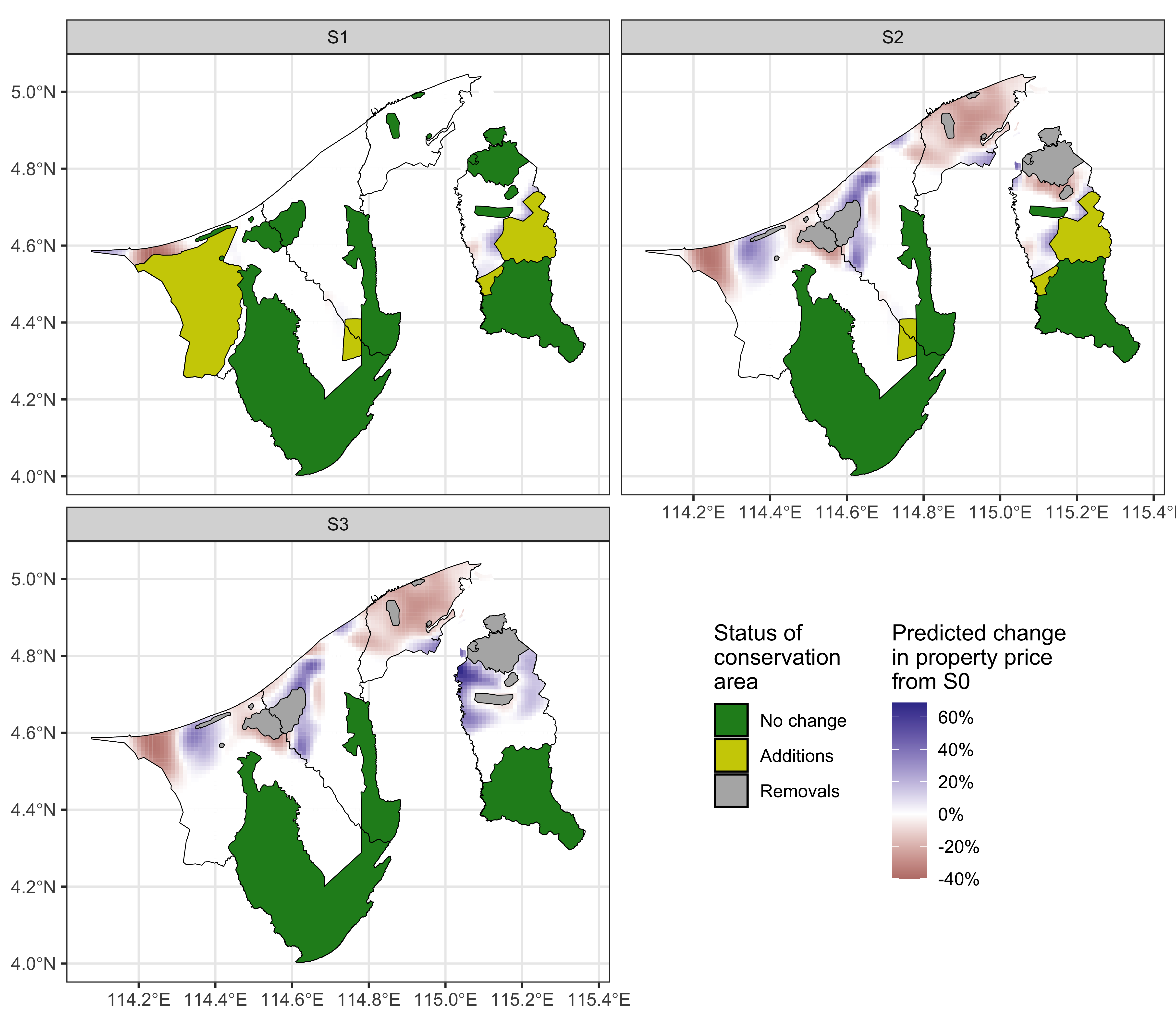
• Scenario 0 (S0): No changes are made to forest reserves, including the proposed gazetted areas, maintaining the current forest reserve coverage at 41%.

• Scenario 1 (S1): An increase in protected areas, with proposed zones being designated as forest reserves, raising the total protected area from 41% to 57%.

• Scenario 2 (S2): A reconfiguration of forest reserve locations while keeping the total protected area constant at 41%.

• Scenario 3 (S3): A reduction in protected areas from 41% to 34%, allowing for potential development within these previously conserved zones.

Figure 2: Map of Brunei Darussalam showing the location of forest reserves. Sample locations of 1,000 properties are depicted, showing a high concentration of population along the coastal areas and as well in the vicinity of the capital city of Bandar Seri Begawan (indicated by the red point).

In order to utilise the sparse GP model for scenario analysis, we first describe some feature engineering steps that are necessary to prepare the data for the model. Concerning the spatial location of the data points, these are geocoded with an areal location in Brunei (village or kampong level resolution). Since these spatial areas are not conducive for direct use in the model, we obtained a random sample from this area and used the X and Y coordinates as an approximate location of the house. With several observations relating to the same spatial area, this would likely have the same effect as using the centroid of the spatial area, with the added benefit of interpolating over the entire spatial area.

Next, the categorical variable property type is hot-encoded to create dummy variables for each property type. The listing date, in the format of “year-quarter” is converted to numeric format by assigning a unique number to each quarter-year in running order. This, together with other continuous variables (X, Y, built-up area), are standardised to have zero mean and unit variance. The output variable price is log-transformed to ensure that the model is not overly sensitive to extreme values, and is quite common practice for these types of analyses.

As the interest is in determining changes to property prices under different conservation scenarios, we calculate a conservation proximity variable, which is simply the distance from each property to the nearest point of the conservation area boundary in the current scenario. This feature will likely play a crucial role in the model.

Considering the different kinds of variables in the dataset, we use a combination of kernels to capture different aspects of the data. In particular, the squared exponential (or radial basis) kernel with differing lengthscales are used for the continuous variables X, Y, built up area and conservation proximity. The Matérn kernel with \(\nu=5/2\) was applied to the time variable. In theory it can adapt better to irregularities in data, which might be suitable for economic or housing data that can experience sudden changes due to external factors. To account for the categorical variable, we use the coregionalize kernel designed to handle multiple outputs or grouped data by modelling correlations between these outputs or groups.

Figure 3: An illustration of the feature engineering process outlining variables used in the GP regression.

The dataset was split into training and validation sets, with 80% of the data used for training and the remaining 20% for validation. The GPy library in Python was used to build the sparse GP model, with the inducing points set to 1000. The model was trained until convergence, which was assessed by the non-change in the marginal likelihood. The mean squared error (MSE) for the training sample was found to be 0.0624, while the MSE for the test sample was 0.0585.

The trained model was then used to predict property prices under the different scenarios. In order to achieve this, the map of Brunei was gridded into cells of size 0.01 degrees, which is approximately 1 km by 1 km. Cells that intersected with the Brunei boundary were retained, resulting in 5,210 cells. The centroid of these cells were used as the location to be predicted. In addition, the property characteristics were set to an average detached house’s characteristics, roughly 2,500 square feet in built-up area. The conservation proximity was then calculated for each data point. The time period of prediction was set to the latest date available (2023 Q3).

Using the described prediction data set, we obtain predicted prices under Scenarios S0 to S3. The main interest will be changes to property prices so therefore the absolute predicted values themselves, and therefore the prediction inputs, are not too important. Specifically, the relative change (in percent) to status quo scenario S0 was calculated for each of S1, S2, and S3. The results are shown as a heatmap in Figure 4. The average change for each of Brunei’s four districts, weighted by household density from the 2021 census data, is also calculated and tabulated in Table 2.

Figure 4: Heatmap of relative changes (S0 baseline) in property prices under different conservation scenarios. Green areas indicate status-quo conservation areas. Yellow areas indicate addition of conservation areas, while gray areas are removed areas.

Table 2: Average relative weighted change in property prices under different conservation scenarios for each district in Brunei.

District	Average price under S0	S1	S2	S3
Belait	$340,000	-14.72%	-8.65%	-8.65%
Tutong	$229,000	0.00%	-0.55%	-0.55%
Brunei Muara	$326,000	0.00%	-19.08%	-19.08%
Temburong	$224,000	0.37%	-0.09%	19.48%

Under S1, where the conservation area is increased, the property prices are predicted to be stable in most areas, but a decrease of about 15% is seen in the Belait area. An increase in conservation area in the district indeed restricts the supply of land available for residential construction, thereby decreasing the potential for capitalizing on land value through development. As a result, property prices are expected to decrease (Hardie et al., 2007). Under S2, where the conservation area is reconfigured, the price surface of Brunei experiences either an increase or a decrease depending on the location. Similar to S1, the Belait populous region experiences a decrease, however the Lumut area sees an increase. The latter seems to be a response to the removal of the nearby Anduki forest reserve. A similar effect, though smaller, is seen in the Tutong region due to the removal of the Andulau forest reserve. More prominently, the removal of the Berakas forest reserve in the Brunei-Muara region leads to a negative effect averaging -19% on property prices, possibly indicating the importance of having conservation land in a very densely populated region. A similar effect was seen in the San Francisco Bay area (Farja, 2017). The effects of S3, i.e. the reduction in conservation area follows a similar pattern to S2, but the magnitude of change is more pronounced. This is especially apparent in the Temburong region, where property prices are predicted to increase by as much as 20% on average. Reduction in conservation areas can spur property price increases by making more land available for development and infrastructure improvements, which support the burgeoning eco-tourism sector in Temburong. Indeed, research has suggested that green-infrastructure development can lead to increased property prices (Fauk & Schneider, 2023; Hsu & Chao, 2022). With investment and boosts to local economies, properties are more valued through increased demand and speculative interest.

5 Conclusion

To conclude, Gaussian Processes have been demonstrated to be an invaluable and powerful tool for spatial data analysis, offering the flexibility and user-friendliness required for complex supervised learning tasks. Their application in urban planning is particularly promising, as they allow for the incorporation of economic considerations into decision-making processes, leading to more informed and sound strategies for urban development.

Despite the notable computational complexities associated with traditional GPs, advancements in technology have given rise to the sparse Gaussian Process method, which mitigates these challenges by optimizing model complexity and computational resources. The sparse GP methodology stands as a testament to the evolution and adaptability of statistical modelling tools in addressing data-intensive problems.

The case study presented in this paper, albeit simplistic, serves as a promising proof of concept for the utilization of sparse Gaussian Processes in scenario analysis for urban planning. It effectively demonstrates the potential of GP models in property price estimation and their broader implications for informed urban development. To unlock the full predictive capabilities of these models and facilitate even more precise insights, the incorporation of a richer dataset is essential. This dataset should include a diverse array of features such as property quality indicators – age of the property, land size, and conditions – alongside neighbourhood and locational attributes like proximity to amenities, road networks, and places of attraction. As we continue to refine these models by integrating these comprehensive features, Gaussian Processes are poised to significantly influence the development of sustainable and economically viable urban environments, aligning with the objectives of Sustainable Development Goal 11.

Acknowledgements

The authors thank Atikah Farhain Yahya, Hafeezul Waezz Rabu, and Amira Barizah Noorosmawie for their invaluable assistance with data collection and processing.

References

Chuweni, N. N., Fauzi, N. S., Che Kasim, A., Mayangsari, S., & Wardhani, N. K. (2024). Assessing the effect of housing attributes and green certification on Malaysian house price. International Journal of Housing Markets and Analysis. https://doi.org/10.1108/IJHMA-10-2023-0145

Csató, L. (2002). Gaussian processes: Iterative sparse approximations [PhD thesis, Citeseer]. https://citeseerx.ist.psu.edu/document?repid=rep1&type=pdf&doi=9e04c1e666e84d466ba4d3e0ec2b3ea71a6eedf0

Dede, O. M. (2016). The Analysis of Turkish Urban Planning Process Regarding Sustainable Urban Development. In M. Ergen (Ed.), Sustainable Urbanization. InTech. https://doi.org/10.5772/63271

Farja, Y. (2017). Price and distributional effects of privately provided open space in urban areas. Landscape Research, 42(5), 543–557. https://doi.org/10.1080/01426397.2016.1250874

Fauk, T., & Schneider, P. (2023). Does Urban Green Infrastructure Increase the Property Value? The Example of Magdeburg, Germany. Land, 12(9), 1725. https://doi.org/10.3390/land12091725

Forestry Dept. (2014). The 5th National Report to the Convention on Biological Diversity. The Forestry Department, Ministry of Industry and Primary Resources.

Hardie, I., Lichtenberg, E., & Nickerson, C. J. (2007). Regulation, Open Space, and the Value of Land Undergoing Residential Subdivision. Land Economics, 83(4), 458–474. https://doi.org/10.3368/le.83.4.458

Hensman, J., Fusi, N., & Lawrence, N. D. (2013). Gaussian Processes for Big Data. In A. Nicholson & P. Smyth (Eds.), Uncertainty in Artificial Intelligence (UAI). Proceedings of the twenty-ninth conference.

Hsu, K.-W., & Chao, J.-C. (2022). The Impact of Urban Green-infrastructure Development on the Price of Surrounding Real Estate: A Case Study of Taichung City’s Central District. IOP Conference Series: Earth and Environmental Science, 1006, 012012. https://iopscience.iop.org/article/10.1088/1755-1315/1006/1/012012/meta

Ishida, S., & Bergsma, W. (2023, August 2). Efficient and Interpretable Additive Gaussian Process Regression and Application to Analysis of Hourly-recorded NO₂ Concentrations in London. http://arxiv.org/abs/2305.07073

Jamil, H. (2024). A spatio-temporal analysis of property prices in Brunei Darussalam. https://doi.org/10.13140/RG.2.2.32533.74720

Jamil, H., & Bergsma, W. (2019, November 30). Iprior: An R Package for Regression Modelling using I-priors. https://doi.org/10.48550/arXiv.1912.01376

Johnson, M. P. (2007). Planning Models for the Provision of Affordable Housing. Environment and Planning B: Planning and Design, 34(3), 501–523. https://doi.org/10.1068/b31165

Kropp, W. W., & Lein, J. K. (2013). Research Articles: Scenario Analysis for Urban Sustainability Assessment: A Spatial Multicriteria Decision-Analysis Approach. Environmental Practice, 15(2), 133–146. https://doi.org/10.1017/S1466046613000045

Matthews, A. G. de G., van der Wilk, M., Nickson, T., Fujii, Keisuke., Boukouvalas, A., León-Villagrá, P., Ghahramani, Z., & Hensman, J. (2017). GPflow: A Gaussian process library using TensorFlow. Journal of Machine Learning Research, 18(40), 1–6. http://jmlr.org/papers/v18/16-537.html

Mironiuc, M., Ionașcu, E., Huian, M. C., & Țaran, A. (2021). Reflecting the Sustainability Dimensions on the Residential Real Estate Prices. Sustainability, 13(5), 2963. https://doi.org/10.3390/su13052963

Rasmussen, C. E., & Williams, C. K. I. (2006). Gaussian processes for machine learning. (pp. I–XVIII, 1–248). MIT Press.

Schoeman, I. M. (2019). Infrastructure assessment as a mechanism to enhance spatial and strategic planning and decision making in determining development priorities within urban areas in developing countries. International Journal of Transport Development and Integration, 3(1), 79–93. https://doi.org/10.2495/TDI-V3-N1-79-93

Shrestha, O., Forsyth, O., Sihotang, M., Sihotang, M. M., & Walsham, S. (2022). Assessing the Socio-Economic Impact of Infrastructure Development on Local Communities: A Mixed-Methods Approach. Jurnal Sosial, Sains, Terapan Dan Riset (Sosateris), 11(1), 1–8. https://doi.org/10.35335/3xahcj54

Snelson, E., & Ghahramani, Z. (2005). Sparse Gaussian processes using pseudo-inputs. Advances in Neural Information Processing Systems, 18. https://proceedings.neurips.cc/paper/2005/hash/4491777b1aa8b5b32c2e8666dbe1a495-Abstract.html

Titsias, M. (2009). Variational learning of inducing variables in sparse Gaussian processes. Artificial Intelligence and Statistics, 567–574. https://proceedings.mlr.press/v5/titsias09a.html

United Nations. (2018). SDG 11 issue brief: Make cities and human settlements inclusive, safe, resilient and sustainable. UN Environment Programme. https://wedocs.unep.org/20.500.11822/25763

Footnotes

1. Known as kriging in the field of geostatistics.