To simulate a complex sampling design, our strategy is to generate data for an entire population inspired by a sampling design in education. The population consists of 2,000 schools (Primary Sampling Units, PSU) of three types: “A” (400 units), “B” (1000 units), and “C” (600 units). The school type correlates with the average abilities of its students (explained further below) and therefore gives a way of stratifying the population. Each school is assigned a random number of students from the normal distribution \(\mathop{\mathrm{N}}(500, 125^2)\) (the number then rounded down to a whole number). Students are then assigned randomly into classes of average sizes 15, 25 and 20 respectively for each school type A, B and C. The total population size is roughly \(N=1\) million students. The population statistics is summarised in the table below.
# Make population
pop <- make_population(model_no = 1, return_all = TRUE, seed = 123)| Type | \(N\) | \(N\) | Avg. | SD | Min. | Max. | Avg. | SD | Min. | Max. |
|---|---|---|---|---|---|---|---|---|---|---|
| A | 400 | 200,670 | 501.7 | 96.9 | 253 | 824 | 15.2 | 3.9 | 3 | 36 |
| B | 1,000 | 501,326 | 501.3 | 100.2 | 219 | 839 | 25.7 | 5.0 | 6 | 48 |
| C | 600 | 303,861 | 506.4 | 101.9 | 195 | 829 | 20.4 | 4.4 | 6 | 39 |
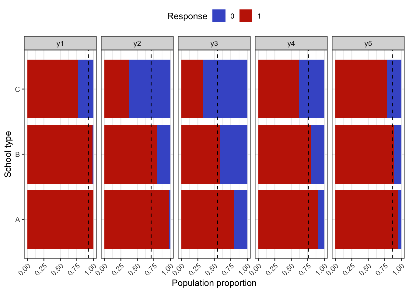
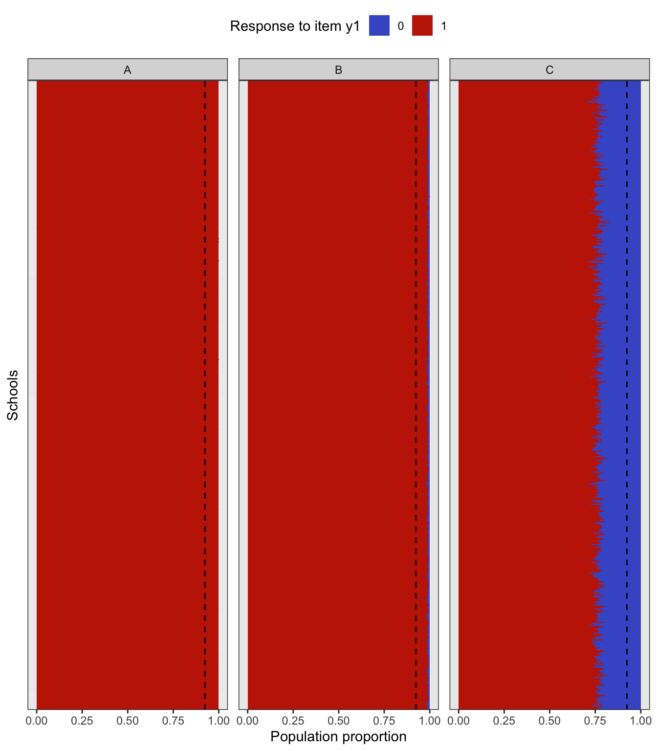
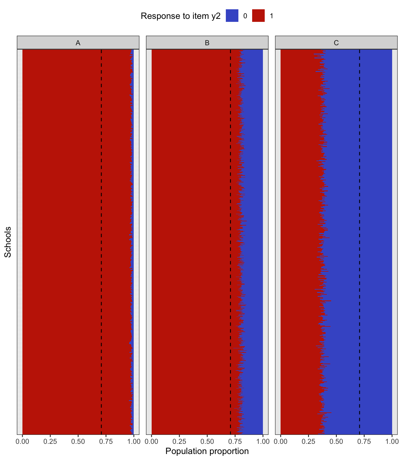
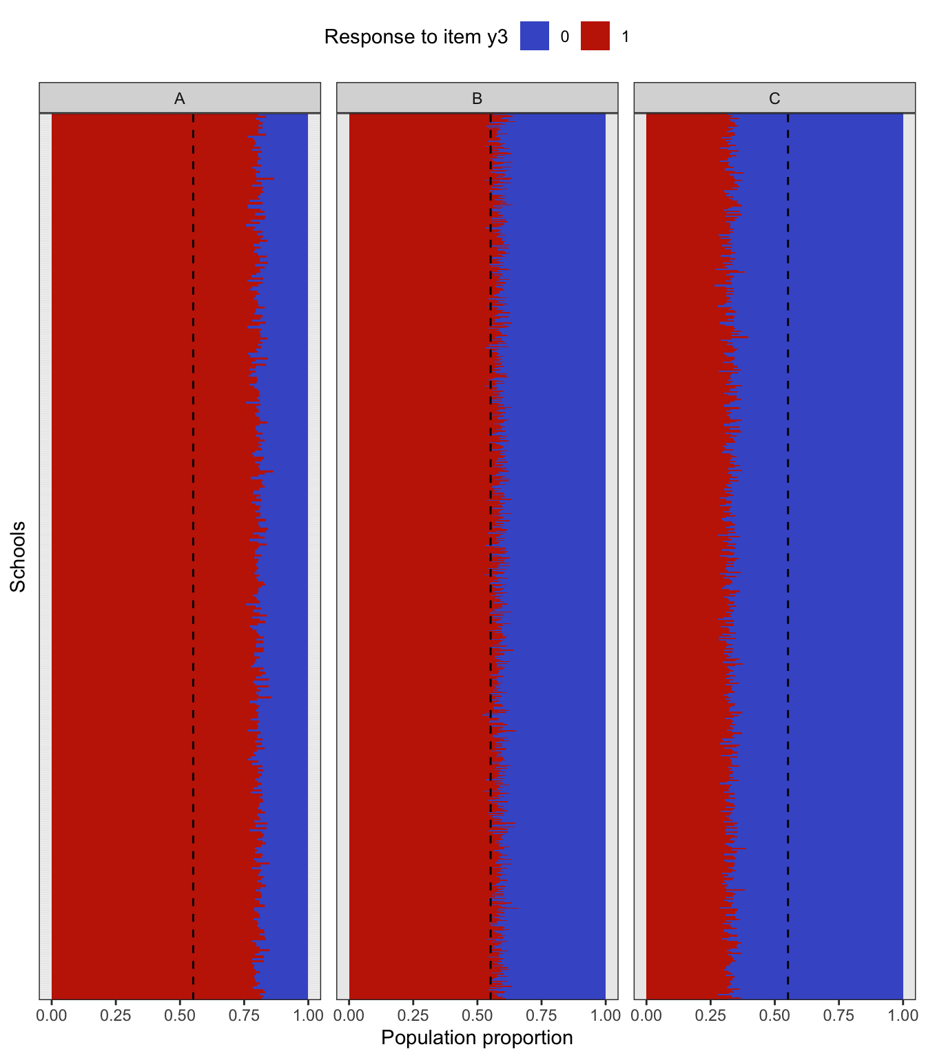
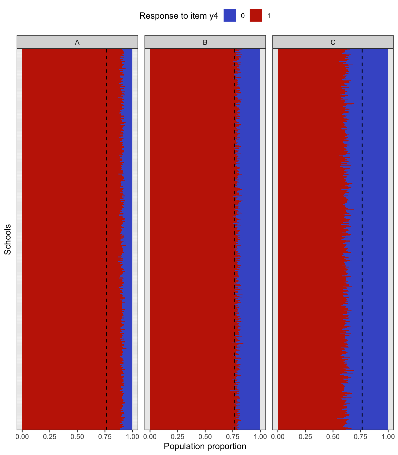
In the factor model, the latent variable \({\boldsymbol\eta}\) represents the abilities of each individual student, and it is used as a stratifying variable in the following way. For each individual \(h=1,\dots,N\), let \({\boldsymbol\eta}_h\) represent the vector of latent abilities generated from \(N_q({\mathbf 0}, {\boldsymbol\Psi})\) as described in a previous article. Define \(z_h=\sum_{j=1}^q \eta_{jh}\), which is now a normal random variate centered at zero. If all the correlations in \({\boldsymbol\Psi}\) are positive, then \(z_h\) has variance at least \(q\). Students are then arranged in descending order of \(z_h\), and based on this arrangement assigned to the school type A, B or C respectively. If the observed variables \(y\) are test items, this would suggest that school type A would consist of ‘high’ ability students, type B ‘medium’ ability student, and type C ‘low’ ability students. Note that the actualised item responses are further subjected to random errors \(\epsilon\).
Probability-based sample
A probability based sampling procedure may be implemented in one of three ways described below.
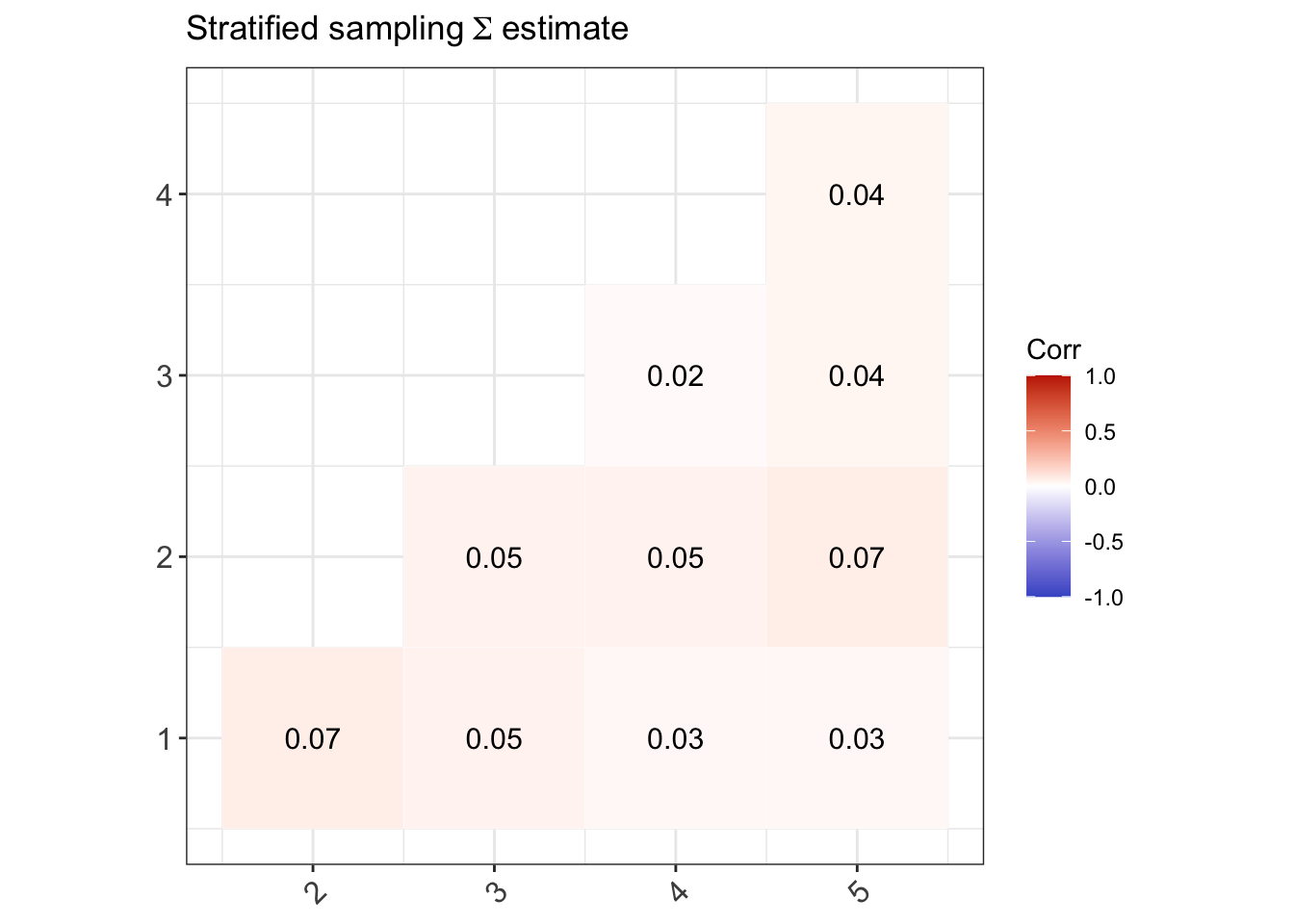
Stratified sampling
From each school type (strata), select 1000 students (PSU) using SRS. Let \(N_a\) be the total number of students in stratum \(a\in\{1,2,3\}\). Then the probability of selection of a student in stratum \(a\) is \(\Pr(\text{selection}) = \frac{1000}{N_a}\). The total sample size is \(n= 3 \times 1000 = 3000\).
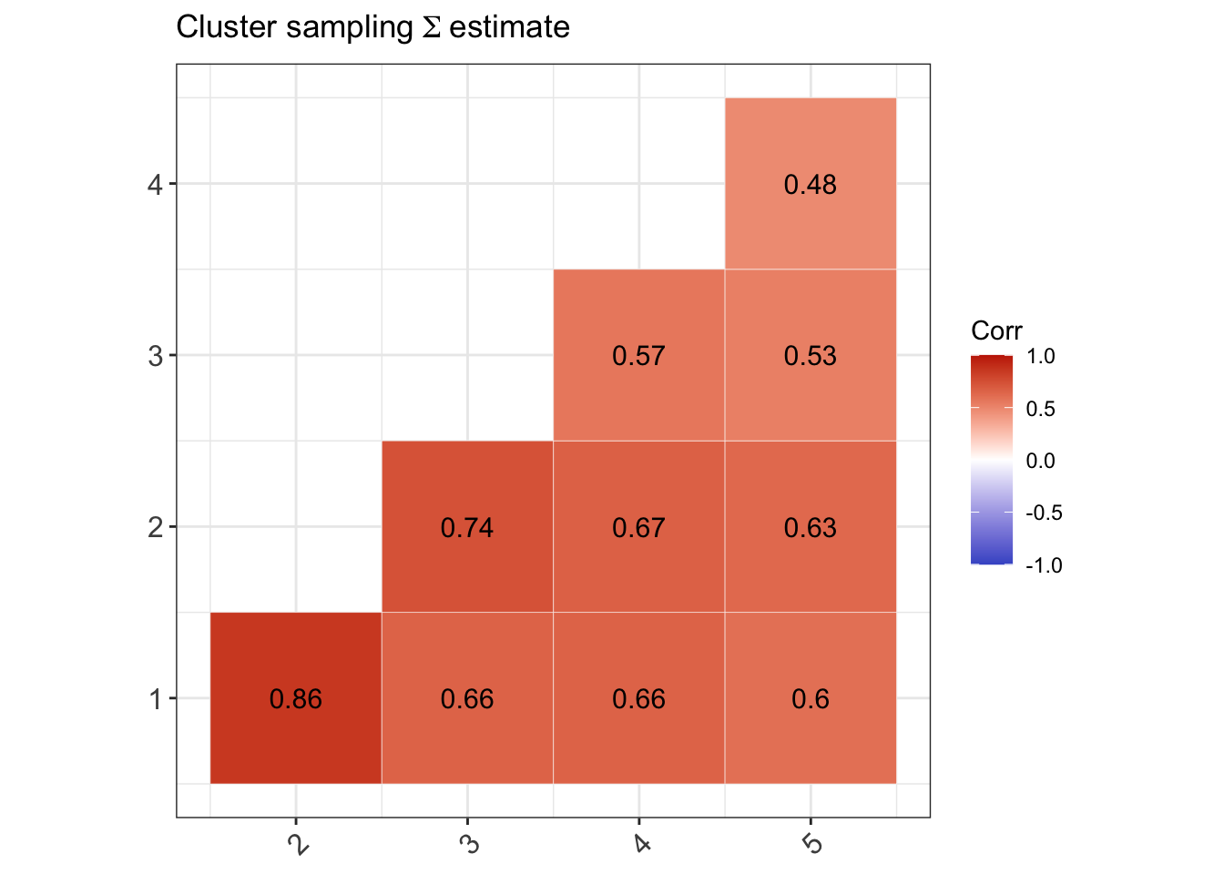
Two-stage cluster sampling
Select 140 schools (PSU; clusters) using probabilities proportional to size (PPS). For each school, select one class by SRS, and all students in that class are added to the sample. The probability of selection of a student in PSU \(b=1,\dots,2000\) is then \[ \Pr(\text{selection}) = \Pr(\text{weighted school selection}) \times \frac{1}{\# \text{ classes in school }b}. \] The total sample size will vary from sample to sample, but on average will be \(n = 140 \times 21.5 = 3010\), where \(\frac{15 \times 400 + 25 \times 1000 + 20 \times 600}{3} = 21.5\) is the average class size per school.
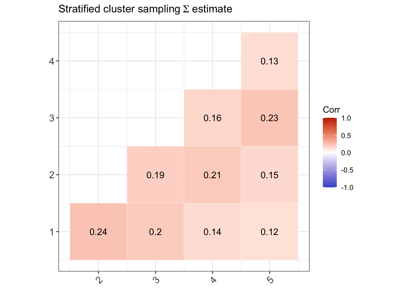
Two-stage stratified cluster sampling
For each school type (strata), select 50 schools using SRS. Then, within each school, select 1 class by SRS, and all students in that class are added to the sample. The probability of selection of a student in PSU \(b\) from school type \(a\) is \[ \Pr(\text{selection}) = \frac{50}{\# \text{ schools of type } a} \times \frac{1}{\# \text{ classes in school }b}. \] Here, the expected sample size is \(n=50 \times (15 + 25 + 20) = 3000\).
Generating the population data
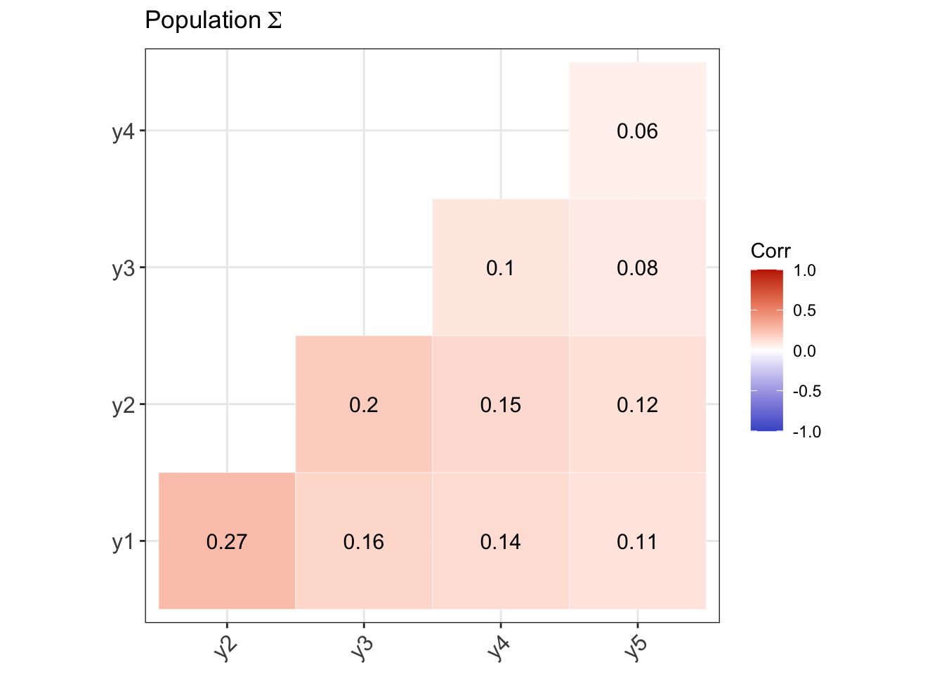
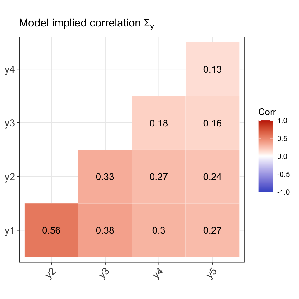
For the purposes of checking the data generation process, we will use Model 1 parameters to generate the response patterns. That is, we assume a 1 factor model with \(p=5\) observed response items. The true model parameter values \({\boldsymbol\theta}\) (loadings and thresholds) are as follows:
#> lambda1 lambda2 lambda3 lambda4 lambda5    tau1    tau2    tau3    tau4    tau5
#>    0.80    0.70    0.47    0.38    0.34   -1.43   -0.55   -0.13   -0.72   -1.13
Comparison of population and model-implied moments
# Univariate moments (model-implied)
round(pi1, 4)
#>     y1     y2     y3     y4     y5
#> 0.9236 0.7088 0.5517 0.7642 0.8708

# Univariate moments (population statistics)
round(prop1, 4)
#>     y1     y2     y3     y4     y5
#> 0.9240 0.7083 0.5515 0.7643 0.8709

# Errors (percentage)
round((prop1 - pi1) / pi1 * 100, 2)
#>    y1    y2    y3    y4    y5
#>  0.04 -0.07 -0.03  0.01  0.01
Model fit
# Comparison of lambda values
round(coef(fit), 2)[1:5]
#> eta1=~y1 eta1=~y2 eta1=~y3 eta1=~y4 eta1=~y5
#>     0.80     0.70     0.47     0.38     0.34
true_vals[1:5]
#> lambda1 lambda2 lambda3 lambda4 lambda5
#>    0.80    0.70    0.47    0.38    0.34

# Comparison of threshold values
round(coef(fit), 2)[-(1:5)]
#> y1|t1 y2|t1 y3|t1 y4|t1 y5|t1
#> -1.43 -0.55 -0.13 -0.72 -1.13
true_vals[-(1:5)]
#>  tau1  tau2  tau3  tau4  tau5
#> -1.43 -0.55 -0.13 -0.72 -1.13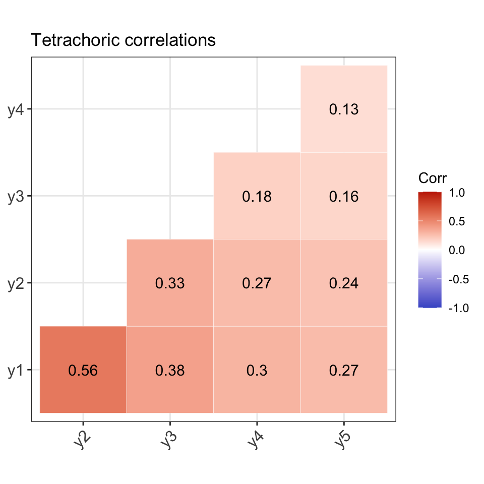

Performing a complex sampling procedure
There are three functions that perform the three complex sampling procedures described earlier.
# Stratified sampling
(samp1 <- gen_data_bin_complex1(population = pop, seed = 123))
#> # A tibble: 3,000 × 9
#>    type  school class    wt y1    y2    y3    y4    y5
#>    <chr> <chr>  <chr> <dbl> <ord> <ord> <ord> <ord> <ord>
#>  1 A     A1     A1ab  0.599 1     1     1     1     1
#>  2 A     A1     A1y   0.599 1     1     1     1     1
#>  3 A     A10    A10a  0.599 1     1     1     1     1
#>  4 A     A10    A10b  0.599 1     1     1     0     1
#>  5 A     A10    A10i  0.599 1     1     1     1     1
#>  6 A     A10    A10s  0.599 1     1     1     1     0
#>  7 A     A101   A101g 0.599 1     1     0     1     1
#>  8 A     A101   A101l 0.599 1     1     1     1     1
#>  9 A     A101   A101q 0.599 1     1     0     1     1
#> 10 A     A101   A101v 0.599 1     1     1     1     1
#> # ℹ 2,990 more rows

# Two-stage cluster sampling
(samp2 <- gen_data_bin_complex2(population = pop, seed = 123))
#> # A tibble: 3,155 × 9
#>    type  school class    wt y1    y2    y3    y4    y5
#>    <chr> <chr>  <chr> <dbl> <ord> <ord> <ord> <ord> <ord>
#>  1 A     A100   A100l  1.48 1     1     1     1     1
#>  2 A     A100   A100l  1.48 1     1     0     1     1
#>  3 A     A100   A100l  1.48 1     1     1     1     1
#>  4 A     A100   A100l  1.48 1     1     1     0     1
#>  5 A     A100   A100l  1.48 1     1     1     1     1
#>  6 A     A100   A100l  1.48 1     1     1     1     1
#>  7 A     A100   A100l  1.48 1     1     0     1     1
#>  8 A     A100   A100l  1.48 1     1     1     1     0
#>  9 A     A100   A100l  1.48 1     1     0     0     1
#> 10 A     A100   A100l  1.48 1     1     1     1     1
#> # ℹ 3,145 more rows

# Two-stage stratified cluster sampling
(samp3 <- gen_data_bin_complex3(population = pop, seed = 123))
#> # A tibble: 3,039 × 9
#>    type  school class    wt y1    y2    y3    y4    y5
#>    <chr> <chr>  <chr> <dbl> <ord> <ord> <ord> <ord> <ord>
#>  1 A     A109   A109b 0.740 1     1     1     1     1
#>  2 A     A109   A109b 0.740 1     1     1     1     1
#>  3 A     A109   A109b 0.740 1     1     1     0     1
#>  4 A     A109   A109b 0.740 1     1     1     1     1
#>  5 A     A109   A109b 0.740 1     1     1     1     1
#>  6 A     A109   A109b 0.740 1     1     1     0     1
#>  7 A     A109   A109b 0.740 1     1     1     1     1
#>  8 A     A109   A109b 0.740 1     1     1     1     1
#>  9 A     A109   A109b 0.740 1     1     0     1     1
#> 10 A     A109   A109b 0.740 1     1     1     1     1
#> # ℹ 3,029 more rows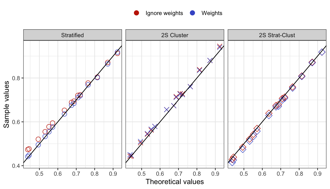
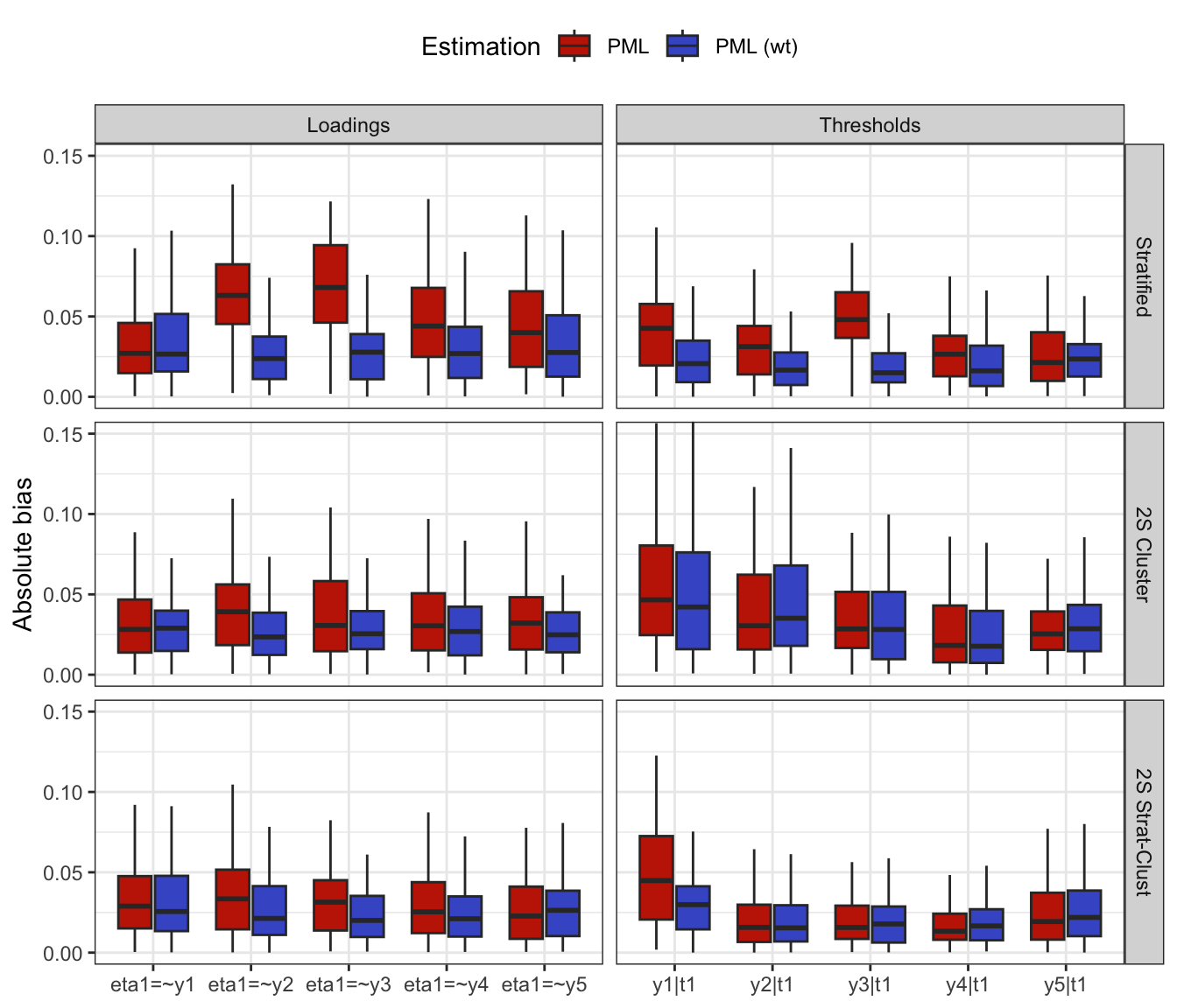
Check bias in model fit
To check the bias in model fit, do the following:
Generate data sets using
gen_data_bin_complex()for the stratified, cluster, and stratified cluster methods.Fit the factor model using lavaan and compare the estimates with the true parameter values
true_vals.Repeat steps 1 & 2 a total of 1,000 times.
Estimating the multinomial covariance matrix
Let \({\mathbf p}\) be the \(R \times 1\) vector of sample proportions (of response patterns) corresponding to the vector of population proportions \({\boldsymbol\pi}\). Assuming iid observations, \[\begin{equation} \sqrt n ({\mathbf p}- {\boldsymbol\pi}) \xrightarrow{\text D}{\mathop{\mathrm{N}}}_{R}({\mathbf 0},{\boldsymbol\Sigma}), \tag{1} \end{equation}\] where \({\boldsymbol\Sigma}= \mathop{\mathrm{diag}}({\boldsymbol\pi}) - {\boldsymbol\pi}{\boldsymbol\pi}^\top\). Under a simple random sampling procedure, the \({\boldsymbol\Sigma}\) may be estimated using \(\hat{\boldsymbol\Sigma}= \mathop{\mathrm{diag}}(\hat{\boldsymbol\pi}) - \hat{\boldsymbol\pi}\hat{\boldsymbol\pi}^\top\), where \(\hat{\boldsymbol\pi}\) are the estimated value of the population proportions based on the null hypothesis being tested \(H_0: {\boldsymbol\pi}= {\boldsymbol\pi}({\boldsymbol\theta})\).
Under a complex sampling procedure, the proportions appearing in (1) should be replaced by the weighted version with elements \[\begin{equation} {\mathbf p}_r = \frac{\sum_h w_h [{\mathbf y}^{(h)} = {\mathbf y}_r]}{\sum_h w_h}, \hspace{2em} r=1,\dots,R. \end{equation}\] For convenience, we may do a total normalisation of the weights so that \(\sum_h w_h=n\), the sample size. Under suitable conditions, the central limit theorem in (1) still applies, although the covariance matrix \({\boldsymbol\Sigma}\) need not now take a multinomial form.
We now discuss how to estimate \({\boldsymbol\Sigma}\) from a stratified multistage sample scheme where the strata are labelled \(a=1,\dots,N_S\) and the PSUs are labelled \(b=1,\dots,n_a\), where \(n_a\) is the number of PSUs selected in stratum \(a\). Let \({\mathcal S}_{ab}\) be the set of sample units contained within PSU \(b\) within stratum \(a\). Define \[\begin{equation} {\mathbf u}_{ab} = \sum_{h \in {\mathcal S}_{ab}} w_h ({\mathbf y}^{(h)} - \hat{\boldsymbol\pi}). \end{equation}\] One may think of these as the ‘deviations from the mean’ of units in PSU \(b\) within stratum \(a\). Further define \[\begin{equation} \bar{\mathbf u}_a = \frac{1}{n_a} \sum_{b=1}^{n_a} {\mathbf u}_{ab}, \end{equation}\] the average of these deviations in stratum \(a\). Then, a standard estimator of \({\boldsymbol\Sigma}\) is given by \[\begin{equation} \hat{\boldsymbol\Sigma}= \frac{1}{n} \sum_a \frac{n_a}{n_a-1} \sum_b ({\mathbf u}_{ab} - \bar{\mathbf u}_a)({\mathbf u}_{ab} - \bar{\mathbf u}_a)^\top. \end{equation}\]
For the three complex sampling procedures discussed earlier,
(Stratified sampling) There are three strata \(a=1,2,3\) corresponding to the school types, and the PSUs are the individual students within schools in each stratum. An equal size is taken per stratum, so \(n_a=1000\), and thus the sample units \({\mathcal S}_{ab}\) lists out the students from various schools and classes within each stratum \(a\) (there is no sum over \(b\)).
(Two-stage cluster sampling) In this case, there is only 1 stratum, \(n_a=n\) and \({\mathbf u}_a=0\).
- (Two-stage stratified cluster sampling) Same as 1, but the sample units \({\mathcal S}_{ab}\) lists out the students from school \(b\) (from the selected class) within each stratum \(a\).